Download
1 / 31
320 likes | 477 Vues
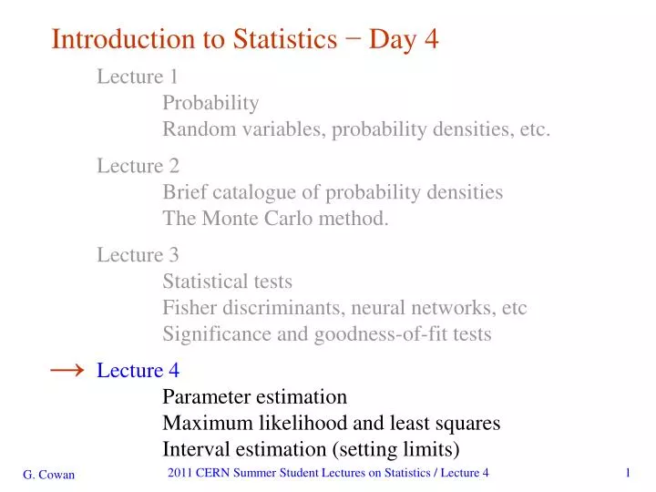
Introduction to Statistics − Day 4. Lecture 1 Probability Random variables, probability densities, etc. Lecture 2 Brief catalogue of probability densities The Monte Carlo method. Lecture 3 Statistical tests Fisher discriminants, neural networks, etc

E N D
Introduction to Statistics − Day 4 Lecture 1 Probability Random variables, probability densities, etc. Lecture 2 Brief catalogue of probability densities The Monte Carlo method. Lecture 3 Statistical tests Fisher discriminants, neural networks, etc Significance andgoodness-of-fit tests Lecture 4 Parameter estimation Maximum likelihood and least squares Interval estimation (setting limits) → 2011 CERN Summer Student Lectures on Statistics / Lecture 4
Parameter estimation The parameters of a pdf are constants that characterize its shape, e.g. random variable parameter Suppose we have a sample of observed values: We want to find some function of the data to estimate the parameter(s): ← estimator written with a hat Sometimes we say ‘estimator’ for the function of x1, ..., xn; ‘estimate’ for the value of the estimator with a particular data set. 2011 CERN Summer Student Lectures on Statistics / Lecture 4
Properties of estimators If we were to repeat the entire measurement, the estimates from each would follow a pdf: best large variance biased We want small (or zero) bias (systematic error): → average of repeated measurements should tend to true value. And we want a small variance (statistical error): →small bias & variance arein general conflicting criteria 2011 CERN Summer Student Lectures on Statistics / Lecture 4
An estimator for the mean (expectation value) Parameter: (‘sample mean’) Estimator: We find: 2011 CERN Summer Student Lectures on Statistics / Lecture 4
The likelihood function Suppose the outcome of an experiment is: x1, ..., xn, which is modeled as a sample from a joint pdf with parameter(s) q: Now evaluate this with the data sample obtained and regard it as a function of the parameter(s). This is the likelihood function: (xi constant) If the xi are independent observations of x ~ f(x;q), then, 2011 CERN Summer Student Lectures on Statistics / Lecture 4
Maximum likelihood estimators If the hypothesized q is close to the true value, then we expect a high probability to get data like that which we actually found. So we define the maximum likelihood (ML) estimator(s) to be the parameter value(s) for which the likelihood is maximum. ML estimators not guaranteed to have any ‘optimal’ properties, (but in practice they’re very good). 2011 CERN Summer Student Lectures on Statistics / Lecture 4
ML example: parameter of exponential pdf Consider exponential pdf, and suppose we have data, The likelihood function is The value of t for which L(t) is maximum also gives the maximum value of its logarithm (the log-likelihood function): 2011 CERN Summer Student Lectures on Statistics / Lecture 4
ML example: parameter of exponential pdf (2) Find its maximum by setting → Monte Carlo test: generate 50 values using t = 1: We find the ML estimate: 2011 CERN Summer Student Lectures on Statistics / Lecture 4
Variance of estimators: Monte Carlo method Having estimated our parameter we now need to report its ‘statistical error’, i.e., how widely distributed would estimates be if we were to repeat the entire measurement many times. One way to do this would be to simulate the entire experiment many times with a Monte Carlo program (use ML estimate for MC). For exponential example, from sample variance of estimates we find: Note distribution of estimates is roughly Gaussian − (almost) always true for ML in large sample limit. 2011 CERN Summer Student Lectures on Statistics / Lecture 4
Variance of estimators from information inequality The information inequality (RCF) sets a lower bound on the variance of any estimator (not only ML): Often the bias b is small, and equality either holds exactly or is a good approximation (e.g. large data sample limit). Then, Estimate this using the 2nd derivative of ln L at its maximum: 2011 CERN Summer Student Lectures on Statistics / Lecture 4
Variance of estimators: graphical method Expand ln L (q) about its maximum: First term is ln Lmax, second term is zero, for third term use information inequality (assume equality): i.e., → to get , change q away from until ln L decreases by 1/2. 2011 CERN Summer Student Lectures on Statistics / Lecture 4
Example of variance by graphical method ML example with exponential: Not quite parabolic ln L since finite sample size (n = 50). 2011 CERN Summer Student Lectures on Statistics / Lecture 4
The method of least squares Suppose we measure N values, y1, ..., yN, assumed to be independent Gaussian r.v.s with Assume known values of the control variable x1, ..., xN and known variances We want to estimate q, i.e., fit the curve to the data points. The likelihood function is 2011 CERN Summer Student Lectures on Statistics / Lecture 4
The method of least squares (2) The log-likelihood function is therefore So maximizing the likelihood is equivalent to minimizing Minimum of this quantity defines the least squares estimator Often minimize c2 numerically (e.g. program MINUIT). 2011 CERN Summer Student Lectures on Statistics / Lecture 4
Example of least squares fit Fit a polynomial of order p: 2011 CERN Summer Student Lectures on Statistics / Lecture 4
Variance of LS estimators In most cases of interest we obtain the variance in a manner similar to ML. E.g. for data ~ Gaussian we have and so 1.0 or for the graphical method we take the values of q where 2011 CERN Summer Student Lectures on Statistics / Lecture 4
Goodness-of-fit with least squares The value of the c2 at its minimum is a measure of the level of agreement between the data and fitted curve: It can therefore be employed as a goodness-of-fit statistic to test the hypothesized functional form l(x; q). We can show that if the hypothesis is correct, then the statistic t = c2min follows the chi-square pdf, where the number of degrees of freedom is nd = number of data points - number of fitted parameters 2011 CERN Summer Student Lectures on Statistics / Lecture 4
Goodness-of-fit with least squares (2) The chi-square pdf has an expectation value equal to the number of degrees of freedom, so if c2min≈ nd the fit is ‘good’. More generally, find the p-value: This is the probability of obtaining a c2min as high as the one we got, or higher, if the hypothesis is correct. E.g. for the previous example with 1st order polynomial (line), whereas for the 0th order polynomial (horizontal line), 2011 CERN Summer Student Lectures on Statistics / Lecture 4
Setting limits Consider again the case of finding n = ns + nb events where nb events from known processes (background) ns events from a new process (signal) are Poisson r.v.s with means s, b, and thus n = ns + nb is also Poisson with mean = s + b. Assume b is known. Suppose we are searching for evidence of the signal process, but the number of events found is roughly equal to the expected number of background events, e.g., b = 4.6 and we observe nobs = 5 events. The evidence for the presence of signal events is not statistically significant. What values of s can we exclude on the grounds that they are incompatible with the data? (→ set limit on s). 2011 CERN Summer Student Lectures on Statistics / Lecture 4
Confidence interval from inversion of a test Confidence intervals for a parameter q can be found by defining a test of the hypothesized value q (do this for all q): Specify values of the data that are ‘disfavoured’ by q (critical region) such that P(data in critical region) ≤ a for a prespecified a, e.g., 0.05 or 0.1. If data observed in the critical region, reject the value q . Now invert the test to define a confidence interval as: set of q values that would not be rejected in a test of sizea (confidence level is 1 - a ). The interval will cover the true value of q with probability ≥ 1 – a. 2011 CERN Summer Student Lectures on Statistics / Lecture 4
Relation between confidence interval and p-value Equivalently we can consider a significance test for each hypothesized value of q, resulting in a p-value, pq.. If pq < a, then reject q. The confidence interval at CL = 1 – a consists of those values of q that are not rejected. E.g. an upper limit on q is the greatest value for which pq ≥ a. In practice find by setting pq = a and solve for q. Still need to choose how to define p-value, e.g., does “incompatible with hypothesis” mean data too high? too low? either? some other criterion? 2011 CERN Summer Student Lectures on Statistics / Lecture 4
Example of an upper limit Find the hypothetical value of s such that there is a given small probability, say, a = 0.05, to find as few events as we did or less: Solve numerically for s = sup, this gives an upper limit on s at a confidence level of 1-a. Example: suppose b = 0 and we find nobs = 0. For 1-a = 0.95, → The interval [0, sup] is an example of a confidence interval, designed to cover the true value of s with a probability 1 - a. 2011 CERN Summer Student Lectures on Statistics / Lecture 4
Poisson mean upper limit (cont.) To solve for sup, can exploit relation to 2 distribution: Quantile of 2 distribution TMath::ChisquareQuantile For low fluctuation of n thisformula can give negative result for sup; i.e. confidence interval is empty! 2011 CERN Summer Student Lectures on Statistics / Lecture 4
More on limit setting Many subtle issues with limits − see e.g. CERN (2000) and Fermilab (2001) confidence limit workshops and PHYSTAT conference proceedings from www.phystat.org. Limit-setter’s phrasebook: CLs (A. Read et al.) Limit based on modified p-value so as to avoid exclusion without sensitivity. Feldman- Confidence intervals from inversion of likelihood- Cousins ratio test (no null intervals, no “flip-flopping”). Bayesian Limits based on Bayesian posterior of e.g. rate parameter (prior: constant, reference, subjective,...) PCL (Power-Constrained Limit) Method for avoiding exclusion without sensitivity; based on power. 2011 CERN Summer Student Lectures on Statistics / Lecture 4
Wrapping up lecture 4 We’ve seen some main ideas about parameter estimation, ML and LS, how to obtain/interpret stat. errors from a fit, and what to do if you don’t find the effect you’re looking for, setting limits. In four days we’ve only looked at some basic ideas and tools, skipping many important topics. Keep an eye out for new methods, especially multivariate, machine learning, Bayesian methods, etc. 2011 CERN Summer Student Lectures on Statistics / Lecture 4
Extra slides 2011 CERN Summer Student Lectures on Statistics / Lecture 4
An estimator for the variance Parameter: (‘sample variance’) Estimator: We find: (factor of n-1 makes this so) where 2011 CERN Summer Student Lectures on Statistics / Lecture 4
Coverage probability of confidence intervals Because of discreteness of Poisson data, probability for interval to include true value in general > confidence level (‘over-coverage’) 2011 CERN Summer Student Lectures on Statistics / Lecture 4
Upper limit versus b Feldman & Cousins, PRD 57 (1998) 3873 b If n = 0 observed, should upper limit depend on b? Classical: yes Bayesian: no FC: yes 2011 CERN Summer Student Lectures on Statistics / Lecture 4
Upper limits for mean of Gaussian (unknown) true mean → measurement → 2011 CERN Summer Student Lectures on Statistics / Lecture 4
Coverage probability for Gaussian problem 2011 CERN Summer Student Lectures on Statistics / Lecture 4