Download
1 / 23
230 likes | 423 Vues
Production And Cost in the Long Run. In the long run, costs behave differently Firm can adjust all of its inputs in any way it wants In the long run, there are no ___ inputs or ___ costs All inputs and all costs are ______

E N D
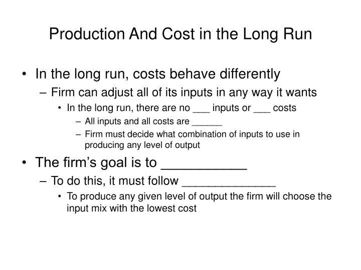
Production And Cost in the Long Run • In the long run, costs behave differently • Firm can adjust all of its inputs in any way it wants • In the long run, there are no ___ inputs or ___ costs • All inputs and all costs are ______ • Firm must decide what combination of inputs to use in producing any level of output • The firm’s goal is to ___________ • To do this, it must follow ______________ • To produce any given level of output the firm will choose the input mix with the lowest cost
Production And Cost in the Long Run • Long-run total cost • The cost of producing each quantity of output when the least-cost input mix is chosen in the long run • Long-run average total cost • The cost per unit of output in the long run, when all inputs are variable • The long-run average total cost (LRATC) • Cost per unit of output in the long-run
The Relationship Between Long-Run And Short-Run Costs • For some output levels, LRTC is ______ than TC • Long-run total cost of producing a given level of output can be less than or equal to, but never greater than, short-run total cost (LRTC ≤ TC) • Long-run average cost of producing a given level of output can be less than or equal to, but never greater than, short–run average total cost (LRATC ≤ ATC)
Average Cost And Plant Size • Plant • Collection of fixed inputs at a firm’s disposal • Can distinguish between the long run and the short run • In the long run, the firm can change the size of its plant • In the short run, it is stuck with its current plant size • ATC curve tells us how average cost behaves in the short run, when the firm uses a plant of a given size • To produce any level of output, it will always choose that ATC curve—among all of the ATC curves available—that enables it to produce at lowest possible average total cost • This insight tells us how we can graph the firm’s LRATC curve
Dollars $4.00 3.00 2.00 1.00 30 90 130 161 184 250 300 0 196 Units of Output Figure 7: Long-Run Average Total Cost ATC1 LRATC ATC3 ATC0 ATC2 C D B E A 175 Use 0 automated lines Use 1 automated lines Use 2 automated lines Use 3 automated lines
Graphing the LRATC Curve • A firm’s LRATC curve combines portions of each ATC curve available to firm in the long run • For each output level, firm will always choose to operate on the ATC curve with ________________ • In the short run, a firm can only move along its current ATC curve • However, in the long run it can move from one ATC curve to another by varying the size of its plant • Will also be moving along its LRATC curve
Economics of Scale • Economics of scale • Long-run average total cost _____ as output increases • When an increase in output causes LRATC to decrease, we say that the firm is enjoying economics of scale • The more output produced, the lower the cost per unit • When long-run total cost rises proportionately less than output, production is characterized by economies of scale • LRATC curve slopes ________
Dollars $4.00 3.00 2.00 1.00 130 184 Figure 8: The Shape Of LRATC LRATC 0 Economies of Scale Constant Returns to Scale Diseconomies of Scale Units of Output
Gains From Specialization • One reason for economies of scale is gains from specialization • The greatest opportunities for increased specialization occur when a firm is producing at a relatively low level of output • With a relatively small plant and small workforce • Thus, economies of scale are more likely to occur at lower levels of output
More Efficient Use of Lumpy Inputs • Another explanation for economies of scale involves the “lumpy” nature of many types of plant and equipment • Some types of inputs cannot be increased in tiny increments, but rather must be increased in large jumps • Plant and equipment must be purchased in large lumps • Low cost per unit is achieved only at high levels of output • Making more efficient use of lumpy inputs will have more impact on LRATC at low levels of output • When these inputs make up a greater proportion of the firm’s total costs • At high levels of output, the impact is smaller
Diseconomies of Scale • Long-run average total cost _______ as output increases • As output continues to increase, most firms will reach a point where bigness begins to cause problems • True even in the long run, when the firm is free to increase its plant size as well as its workforce • When long-run total cost rises more than in proportion to output, there are diseconomies of scale • LRATC curve slopes ________________ • While economies of scale are more likely at low levels of output • Diseconomies of scale are more likely at higher output levels
Constant Returns To Scale • Long-run average total cost is ______ as output increases • When both output and long-run total cost rise by the same proportion, production is characterized by constant returns to scale • LRATC curve is ___ • In sum, when we look at the behavior of LRATC, we often expect a pattern like the following • Economies of scale (decreasing LRATC) at relatively low levels of output • Constant returns to scale (constant LRATC) at some intermediate levels of output • Diseconomies of scale (increasing LRATC) at relatively high levels of output • This is why LRATC curves are typically U-shaped
Using the Theory: Long Run Costs, Market Structure and Mergers • The number of firms in a market is an important aspect of market structure—a general term for the environment in which trading takes place • What accounts for these differences in the number of sellers in the market? • Shape of the LRATC curve plays an important role in the answer
LRATC and the Size of Firms • The output level at which the LRATC first hits bottom is known as the minimum efficient scale (MES) for the firm • Lowest level of output at which it can achieve minimum cost per unit • Can also determine the maximum possible total quantity demanded by using market demand curve • Applying these two curves—the LRATC for the typical firm, and the demand curve for the entire market—to market structure • When the MES is small relative to the maximum potential market • Firms that are relatively small will have a cost advantage over relatively large firms • Market should be populated by many small firms, each producing for only a tiny share of the market
LRATC and the Size of Firms • There are significant economies of scale that continue as output increases • Even to the point where a typical firm is supplying the maximum possible quantity demanded • This market will gravitate naturally toward monopoly • In some cases the MES occurs at 25% of the maximum potential market • In this type of market, expect to see a few large competitors • There are significant lumpy inputs that create economies of scale • Until each firm has expanded to produce for a large share of the market
Dollars $160 80 1,000 3,000 100,000 0 Units per Month Figure 9: How LRATCHelps Explain Market Structure LRATCTypical Firm F E DMarket
Dollars $160 80 100,000 0 Units per Month Figure 9: How LRATCHelps Explain Market Structure LRATCTypical Firm DMarket
Dollars $200 80 100,000 25,000 0 Units per Month Figure 9: How LRATCHelps Explain Market Structure LRATCTypical Firm H F E DMarket
Dollars $160 80 1,000 10,000 100,000 0 Units per Month Figure 9: How LRATCHelps Explain Market Structure LRATCTypical Firm E F DMarket
LRATC and the Size of Firms • The MES of the typical firm in this market is 1,000 units • Lowest output level at which it reaches minimum cost per unit • For firms in this market, diseconomies of scale don’t set in until output exceeds 10,000 units • Since both small and large firms can have equally low average costs with neither having any advantage over the other • Firms of varying sizes can coexist
The Urge To Merge • If by doubling their output, firms could slide down the LRATC curve in Figure 9, and enjoy a significant cost advantage over any other, still-smaller firm, they would • This is a market that is ripe for a merger wave • A sudden merger wave is usually set off by some change in the market • Market structure in general—and mergers and acquisitions in particular—raise many important issues for public policy • Low-cost production can benefit consumers—if it results in lower prices