Download
1 / 26
270 likes | 691 Vues
Progressive Signal Systems. Coordinated Systems. Two or more intersections Signals have a fixed time relationship to one another Progression can be achieved if the offsets between adjacent signals permit continuous operation of groups of vehicles at a planned rate of speed.

E N D
Coordinated Systems • Two or more intersections • Signals have a fixed time relationship to one another • Progression can be achieved if the offsets between adjacent signals permit continuous operation of groups of vehicles at a planned rate of speed
TIME SPACE DIAGRAM Progression Speed Time Red Time Bandwidth Offset = 107 sec Offset = 107 sec Offset = 10 sec Distance
Bandwidth = time in seconds elapsed between the passing of the first and the last vehicle • Progression speed= speed at which the platoon drives through a series of signals without stopping • Slope of the band
D D V = V = 1.47 C 0.735 C Two Basic Types of Progressive System • Simultaneous System • Alternative System Where: V = speed in mph D = signal spacing in feet C = cycle length in seconds
48 mph 48 mph D D D D D 3000 3000 3000 3000 V = V = V = V = V = = = = = = 51 mph 0.735 C 0.735*80
Cycle Lengths • All intersections in system are to have the same cycle length • long enough to provide sufficient capacity at the busiest intersection • System cycle length is determined through a series of steps • determine the minimum (optimum) cycle length at each intersection • as if they are isolated signals
D D C = C = 1.47 V 0.735 V • Speed and signal spacing are entered into the equation and solved for cycle length if the spacings between signals are approximately equal. • Simultaneous System • Alternative System where: V = speed in mph D = signal spacing in feet C = cycle length in seconds
The pattern that has a cycle length closer to, but not less than the “maximum” cycle length is chosen • The cycle length may be selected from a range that has a lower limit calculated as 90% of the “maximum” cycle length
Offsets • Number of seconds or percent of cycle length from the reference base of a time-space diagram to the first green indication • Shown in time-space diagrams • The beginning of the first green from the reference base
Speed of Traffic versus Speed of Progression • Speed of progression • often selected to be the free-flow speed of traffic • Some engineers use it as speed limit. • speed that might be observed when volumes are light and the signals are continuously green on that route • As traffic becomes heavy (peak periods) • traffic speeds tend to drop because of congestion • traffic starting up on a green signal may be stopped by a queue not yet into motion at the next signal downstream
Definitions of Flow, Density & Speed • Flow is defined as the number of vehicles traversing a point of roadway per unit time. Unit: vehicles per hour. • Density is the number of vehicles occupying a given length of lane or roadway averaged over time. Unit: vehicles per mile. • Speed is defined as the distance traversed by a vehicle per unit time. Unit: miles per hour.
q-K-V Relationship Flow (veh/hr) = Density (veh/mile) x Speed (miles/hr) Therefore, q = K x V
q-K-V Curves Flow (veh/hr) Critical Speed Speed (miles/hr) Jam Density Critical Density Density (veh/mile) Flow (veh/hr)
Time Space Diagram for Progression on M-29 80-Second Cycle Length and 45 mph
Telegraph Road Corridor from 12 Mile Road to Maple Road Existing PM Peak Hour
Proposed Progression on Telegraph Road PM PEAK 120 sec Cycle length For 45 mph
Proposed Progression on Telegraph Road PM PEAK 120 sec Cycle length For 35 mph
Proposed Progression on Telegraph Road PM PEAK 90 sec Cycle length For 45 mph
Other Considerations • Traffic Turning into System • Adjustments at End Intersections • Adjustments for Left-Turn Phases • Offsets for Maximum Bandwidths • Offsets for Minimum Stops and Delay
Software Programs • PASSER II- Optimize bandwidths • TRANSYT 7F- Minimizes disutility function • NETSIM- Optimizes synchronization • Synchro- models and optimizes traffic signals • Optimizes to reduce delay • SimTraffic- to check and fine tune signal operations
Synchro Software Program Telegraph Road Corridor 14 Mile Road to Maple Road
SimTraffic Software Program M-29 Intersection in Algonac, MI