Download

1 / 35
360 likes | 989 Vues
Implications of using the HyperSpace Diagonal Counting (HSDC) method for visually representing 3-D shapes By Mallepally Mithun K Reddy Department of Mechanical and Aerospace Engineering Project Defense December 29 th , 2006 Overview Introduction & Motivation Multidimensional Visualization

E N D
Implications of using the HyperSpace Diagonal Counting (HSDC) method for visually representing 3-D shapes By Mallepally Mithun K Reddy Department of Mechanical and Aerospace Engineering Project Defense December 29th, 2006
Overview • Introduction & Motivation • Multidimensional Visualization • Hyper-Space Diagonal Counting (HSDC) • Results • Conclusions • Future Work
Introduction & Motivation • Scientific Visualization • Allows visual representation of data • 2D or 3D graphs • Easy to understand • Multidimensional Data • Difficult to visualize • Not so easy to understand • Numerous methods – different applications
Low order Multidimensional Data High order Multidimensional Data Dimension Reduction Multidimensional Visualization Multidimensional Visualization • Multidimensional Multivariate Visualization (MDMV) • Translate multidimensional data into visual representations • Reduce dimensionality • Dimension Reduction • Some variables can be correlated • Few variables may be irrelevant
Dimension Reduction • Dimension Reduction Techniques • Clustering of variables • Drawbacks • Mostly suitable for linear structures • Computationally expensive • Loss of meaning • Loss of ability to understand the representation intuitively
MDMV Techniques • Techniques designed for a fixed number of variables • Use of color • Animation • Techniques designed for any number of variables • Scatterplots • Chernoff faces – Glyphs • Many others
MDMV Examples Glyphs Scatterplot Matrix
HSDC - Methodology Development • Cantor’s Theory • One-to-one correspondence of points on a line and points on a 2D surface • 2D array of points can be laid flat on a line Array of points on a surface Path through all the points Graphic Proof of Cantor’s Theory
Methodology Development • Points from 3D space – mapped to points on a line • Make an array of points in 3D space • Create a path through the points
Methodology • Similarly, we can map points from an n-dimensional space to unique points on a line • Hyper-Space Diagonal Counting (HSDC) in nD
Relevance • What has any of this to do with visualization? • HSDC allows collapsing multiple dimensions on a single axis • Counting covers each point in a lossless fashion • HSDC – wide breadth of applications • Overarching relationship in variables • No overarching relationship – data already generated • May include exploration of databases to identify trends
Binning technique - explained • To be able to use HSDC for multiobjective problems • Need an index based approach • Binning technique – index based representation • Consider a bi-objective problem
Traditional Pareto Frontier • 245 Pareto points were generated
Binning Technique • Binning Technique – steps involved • Obtain Pareto points • Identify Max. and Min. for each objective to establish a range • Divide ranges into some finite number of bins. Example, objective F1 can be divided into 100 bins, 1 through 100. • Indices of these bins can be plotted along an axis, thus we can have indices of F1 on X-axis and F2 indices on Y-axis • Each Pareto point, previously generated, will fall under some combination of these bins • Represented as a unit cylinder along the third axis • Multiple points may fall under the same set of indices
Binning Technique • Representation of Pareto frontier using binning technique
Binning Technique • Index-based representation of Pareto frontier • Same as traditional Pareto frontier • Small changes in representation – due to discretization • Multiple Pareto points in bins – again, due to discretization • IMPORTANT • Axes enumerate indices • Not actual function values • We can use HSDC for mapping two or more objectives on one axis
Grid Spanning • Spanning the grid • To what diagonal to count – to span the entire grid?
Outline of research - results • Idea – search for extensibility of trends • Procedure • Inspect 2D shapes – observe trends • Straight lines • Circles • Squares/rectangles • Inspect 3D shapes • Cube • Sphere
Straight line – HSDC (10 bins/axis) Y=500X Y=3X Y=0 Y=(-500)X
Conclusions for a straight line • No. of bins needed – depends on the slope • Spread of bins occupied also depends on the slope • Looking at the HSDC plot doesn’t lead us to conclude anything
Circle Radius = 1, Center (2,2) Radius =1, Center (1,1) Radius =2, Center (-2,2) Radius =10, Center (2, -2)
Conclusions for a circle • HSDC plots are the same – independent of radius and center of the circle • If a HSDC plot resembles the one got above – it is that of a circle
Square Square at (0,0), edge = 2 units, inclination with major axis=0 HSDC plot of the adjacent square
Square.. Square at (0,0), edge = 2 units, inclination with major axis=10º Square at (0,0), edge=2 units, inclination with major axis=20º HSDC plot of the above square HSDC plot of the above square
Rectangle (length=5, breadth=1) Inclination with major axis=10º Inclination with major axis=45º
Conclusions about square/rectangle • HSDC plots of square/rectangle of all configurations are similar • The points occur in pairs (similar to a circle but has differences)
Circle vs square HSDC plot of square HSDC plot of circle - Though there is coupling in both the shapes, there is a difference in the spreads
3D shapes -motivation • 3D shapes are extensions of 2D • If similar trends are found, it would mean that there is extensibility and can be extended to n-D objects similarly. • Looking at the HSDC plot of an unknown dataset, one can intuitively visualize the shape by comparing the HSDC plot with that of the known shapes
Cube (Edge 10 units; Inclination with all axes=0º) HSDC plot of cube HSDC plot of square with inclination of 0º - There are similarities in both the figures
Cube (Edge 10 units; inclination with X-axis = 30º) HSDC plot of cube Points are color coded - Similar to the earlier figure - End points in the HSDC space, correspond to end points on the cube
Cube (Edge 10 units; inclination with X-axis = 45º) Points are color coded HSDC plot of cube - Similar to the earlier figure - End points in the HSDC space, correspond to end points on the cube
Sphere (inclination with all axes = 0º) Points on the surface – color coded HSDC plot of the sphere - Similar to the earlier figure - End points in the HSDC space, correspond to end points on the sphere as expected
Conclusions • HSDC method explained • HSDC method applied on • 2D shapes – line, circle, square, rectangle • 3D shapes – cube, sphere • Trends seen in 2D are seen in 3D • Method seems to be extensible to higher dimensions
Future work • Explore hyper-cube and hyper-sphere (more than 4 dimensions) to verify that similar trends are seen • Exploring more shapes will give more insight into the trends