Download
1 / 49
490 likes | 1.01k Vues
Analytical and numerical approximations to the radiative transport equation for light propagation in tissues. Arnold D. Kim School of Natural Sciences University of California, Merced. TexPoint fonts used in EMF. Read the TexPoint manual before you delete this box.: .

E N D
Analytical and numerical approximations to the radiative transport equation for light propagation in tissues Arnold D. Kim School of Natural Sciences University of California, Merced TexPoint fonts used in EMF. Read the TexPoint manual before you delete this box.:
We seek to give an overview of the analytical and numerical approximations used in studying light propagation in tissues. • The theory of radiative transport governs light propagation in tissues. • Typically, one make several simplifying assumptions to the general radiative transport equation. • We wish to become familiar with some of the more common analytical and computational methods used in light propagation in tissues.
Light propagation in tissues is governed by the radiative transport equation. This theory takes into account absorption and scattering due to inhomogeneities.
We have made several assumptions in applying radiative transport theory to light propagation in tissues. • There are no correlations between fields, so the addition of power (not the addition of fields) holds. • The background is homogeneous. • There is no time dependence. • There is no polarization. • In what follows, we discuss each of these assumptions.
There are no correlations between fields, so the addition of power (not the addition of fields) holds. This is the key assumption in radiative transport theory. For a discrete random medium, this assumption corresponds to a medium being sufficiently dilute that scattered fields are not correlated, but dense enough that one can take a continuum limit. For a continuous random medium, the random fluctuations must be relatively small and vary on a scale on the order of the wavelength.
The background is homogeneous. The theory of radiative transport can be extended readily to take into account a varying background refractive index. There have been several theories proposed for this problem. G. Bal [J. Opt. Soc. Am. A 23, 1639-1644 (2006)] has reviewed the existing theories and offered a mathematical explanation for the correct theory.
There is no time dependence. The theory of radiative transport can be extended readily to take into account time dependence (for a sufficiently narrow bandwidth). For ultra-short pulses (broad bandwidth), one may need to consider a two-frequency radiative transport equation. See, for example, A. Ishimaru, J. Opt. Soc. Am. 68, 1045–1050 (1978) and A. C. Fannjiang, C. R. Physique 8, 267-271 (2007).
There is no polarization. The theory of radiative transport can be extended readily to take into account polarization through the so-called Stokes matrix. Here I is a 4-vector containing the Stokes parameters (I, Q, U and V) and S is a 4x4 scattering matrix. Polarization is neglected very often for mathematical simplicity. See M. Moscoso et al, J. Opt. Soc. Am. A 18, 948-960 (2001) and references therein to learn about polarization phenomena used for light propagation in tissues.
We focus our attention on the steady-state (continuous wave), scalar problem. • According to radiative transport theory, there is a diversity of data available from scattered light measurements. • To reach the full potential of diffuse optical tomography and optical molecular imaging, one needs to understand how information is contained in scattered light measurements. • Rather than focus on what technology can offer, we focus on exploiting all we can from simple data sets.
Boundary conditions prescribe the light going into the domain at the boundary surface.
When there is an refractive index mismatch at the boundary, we must include transmission and reflection operators in the boundary condition.
The scattering phase function is assumed often to be rotationally invariant.
Henyey and Greenstein (1941) proposed a simple, one parameter scattering phase function. This scattering phase function model is the one used most commonly for light propagation in tissues. Experimental studies have shown it to work reasonably well at modeling scattered light measurements.
In the near-infrared portion of the spectrum, tissues absorb light weakly and scattering light strongly with a sharp forward peak. W.-F. Cheong et al [IEEE J. Quant. Electron. 26, 2166-2185 (1990)] give several results for values of the optical parameters ma, ms and g (assuming the Henyey-Greenstein model) in tabulated form as well as an explanation for how these estimated values were obtained.
Light is often delivered to and collected from tissues using optical fibers. There are a variety of optical fiber probe designs that deliver light into tissues in different ways. We model different modes for delivering light into tissues through the spatial and directional dependence of the boundary condition.
We characterize optical fiber detectors through the numerical aperture (NA). z y We model a fiber detector measurement as x
Optical fiber detectors measure angular integrals of the specific intensity. • Measurements from other detectors such as charged-coupler device (CCD) cameras are similar even though they measure the spatial variation over a two-dimensional array. • We can obtain directional diversity in measurements by using different optical fibers with different numerical apertures, but that method is not practical. • Some experiments have measured carefully the directional dependence of scattered light using goniometers, but those experiments are not too common.
We consider now several analytical approximations that are used or are useful (we believe) for light propagation in tissues. • PN • Diffusion • Delta-Eddington • Fokker-Planck and extensions
The PN approximation involves expanding the specific intensity in terms of spherical harmonics. See S. Arridge [Inverse Problems 15, R41-R93 (1999)] for the details of this calculation.
The PN approximation has some obvious challenges. The PN approximation reduces the dimensionality of the problem substantially by projecting out the directional dependence. The solution of the radiative transport equation can be discontinuous with respect to W, especially near boundaries (recall how boundary conditions are prescribed). Hence, the spherical harmonics expansion would converge slowly thereby requiring several terms for an accurate approximation. Otherwise, one must prescribe approximate boundary conditions.
We consider specifically the P1 approximation which yields The diffusion approximation is substantially simpler than the radiative transport equation and has been used extensively to model light propagation in tissues.
We can understand better the diffusion approximation by a different derivation.
The diffusion approximation applies to light that has propagated deeply in an optically thick medium. • The specific intensity becomes nearly isotropic due to strong multiple scattering. It is not valid near sources and boundaries (must add boundary layer solutions). • Many have sought extensions of the diffusion approximation to increase its region of validity so that it may apply to a broader range of problems. • Regardless, most state-of-the-art optical tomography and optical molecular imaging reconstructions are based on the diffusion approximation.
The diffusion approximation takes into account that tissues scattering light strongly and absorb light weakly, but it does not take into account explicitly that scattering is sharply peaked in the forward direction. As g ! 1, the diffusion length scale l* = [ms(1-g)]-1 becomes much larger than the scattering mean free path ls = ms-1. When these two scales separate light may scatter multiply over a non-trivial length scale before becoming diffusive.
In the Delta-Eddington approximation, we approximate the scattering phase function by a sum of two parts.
One can derive an alternate diffusion equation by applying the P1 approximation to the modified transport equation using the Delta-Eddington approximation. V. Venugopalanet al [Phys. Rev. E 58, 2395-2407 (1998)] have shown that this modified diffusion equation models scattered light measurements much better than the standard diffusion equation. In particular, they showed improvements for small source-detector separations thereby extending the spatial range of validity.
The Fokker-Planck approximation addresses sharply peaked forward scattering by asymptotic analysis of the scattering operator.
Just as the Delta-Eddington approximation involves two parts, we can add another operation to obtain the Boltzmann-Fokker-Planck approximation. See R. Sanchez and N. McCormick [Transport Theory and Statist. Phys. 12, 129-155 (1983)] for more details about this approximation and solutions to some inverse problems.
We consider now several computational approximations that are used for light propagation in tissues. Computing numerical solutions to the radiative transport equation are challenging due to the large number of independent variables. There are several numerical methods to solve the radiative transport equation. We do not discuss Monte Carlo methods here even though they are used widely for solving direct problems because they are not practical for computational solutions of inverse problems.
There are a variety of methods to treat the direction and spatial variables numerically. • Spatial variables • Finite differences • Finite volumes • Finite elements • Spectral • Directional variables • Spherical harmonics • Finite elements • Discrete ordinate Combining methods for directional and spatial variables leads to different numerical methods.
A comprehensive review of numerical methods for the radiative transport equation is not possible here. Instead, we focus on so-called plane wave solutions and how they can be used to solve inverse problems. Plane wave solutions are general solutions to a homogeneous problem with constant coefficients. These solutions can be used as a basis for numerical computations from which we can compute Green’s function, for example.
Plane wave solutions are special solutions of the radiative transport equation.
We cannot calculate plane wave solutions analytically, so we calculate them numerically using the discrete ordinate method.
We can compute Green’s function as an expansion in plane wave solutions. See A. D. Kim [J. Opt. Soc. Am. A 21, 797-803(2004)] for details of this calculation.
With Green’s function known, we can make use of the general representation formula.
Example: Inverse source problem Under some reasonable assumptions, we can formulate the optical molecular imaging problem as the inverse source problem: Suppose there is a source Q located inside a half-space D = {z > 0} with boundary D = {z = 0} of tissue that is uniformly absorbing and scattering. That is the only source. Can we determine properties of the source only from measurements at the boundary?
We suppose the specific intensity at the boundary is known (i.e. angular data).
According to the general representation formula, the intensity at the boundary is given by
We Fourier transform the reduced problem and substitute Green’s function to obtain
Using orthogonality of plane wave solutions, we can construct non-radiating sources.
We compute special solutions of the reduced problem for an isotropic source. With the reduced problem, we can compute explicit solutions for • Point source • Pixel/voxel source Using these two solutions, we seek the location, size and total strength of a general source. pixel/voxel source -function source
We are working currently on extensions of this idea. • We are formulating a general inverse scattering theory for the radiative transport equation using angular data (with J. Schotland and M. Moscoso). • We have applied these ideas to reconstructing a “thin” obstacle in a half space using flux data (with P. Gonzalez-Rodriguez and M. Moscoso) [AIP 2007 talk]. • We are working with V. Venugopalan (UC Irvine) to validate this theory using experimental data for layered media.
Summary • We have reviewed the theory of radiative transport and how it is applied to problems in light propagation in tissues. • We have discussed some analytical and numerical approximation methods used to study problems of practical interest. • We have discussed plane wave solutions and how they have use for solving inverse problems.
We recommend four books on the subject for those getting started in this field. • K. M. Case and P. F. Zweifel, Linear Transport Theory, (Addison-Wesley, Reading, MA, 1967). • A. Ishimaru, Wave Propagation and Scattering in Random Media, (IEEE Press, New York, 1997). • A. J. Welch and M. J.C. van Gemert (eds), Optical-Thermal Response of Laser-Irradiated Tissue, (Plenum Press, New York, 1995). • H. C. van de Hulst, Multiple Light Scattering: Tables, Formulas, and Applications, (Academic Press, New York, 1980).