Download

1 / 39
390 likes | 866 Vues
Artificial Intelligence Chapter 22. 22. Planning. 22.1 STRIPS Planning Systems. Describing States and Goals. Frame problem (planning of agent actions) state space + situation-calculus approaches Planning states and world states

E N D
Describing States and Goals • Frame problem (planning of agent actions) state space + situation-calculus approaches • Planning states and world states • planning states: data structure that can be changed in ways corresponding to agent actions – state description • world states: fixed states (C) 2000, 2001 SNU CSE Biointelligence Lab
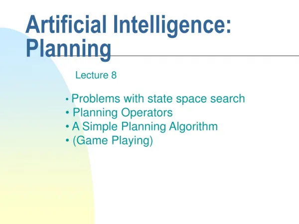
Search process to a goal • Goal wff and variables (x1, x2, …, xn) • goal wffs of the form (x1, x2, …, xn) (x1, x2, …, xn) is written as (x1, x2, …, xn). • Assumption • existential quantification of all of the variables. • the form of a goal is a conjunction of literals • Search methods • attempt to find a sequence of actions that produces a world state described by some state description S, such that S|= • state description satisfies the goal • substitution exists such that is a conjunction of ground literals. • Forward search methods and Backward search methods (C) 2000, 2001 SNU CSE Biointelligence Lab
Forward Search Methods (1) • Actions Operators • based on STRIPS system operator • before-action, after-action state descriptions • A STRIPS operator consists of: 1. A set, PC, of ground literals called the preconditions of the operator. An action corresponding to an operator can be executed in a state only if all of the literals in PC are also in the before-action state description. 2. A set, D, of ground literals called the delete list. 3. A set, A, of ground literals called the add list. (C) 2000, 2001 SNU CSE Biointelligence Lab
STRIPS operators • STRIPS assumption • when we delete from the before-action state description any literals in D and add all of the literals in A, all literals not mentioned in Dcarry over to the after-action state description. • STRIPS rule (an operator schema) • has free variables and ground instances (actual operators) of these rules • example) move(x,y,z) PC: On(x,y)Clear(x)Clear(z) D: Clear(z),On(x,y) A: On(x,z),Clear(y),Clear(F1) (C) 2000, 2001 SNU CSE Biointelligence Lab
Figure 22.2 The application of a STRIPS operator (C) 2000, 2001 SNU CSE Biointelligence Lab
Forward Search Methods (2) • General description of this method • Generate new state descriptions by applying instances of STRIPS rules until a state description is produced that satisfies the goal wff. • One heuristic: identifying and exploiting islands toward which to focus search • make forward search more efficient Figure 22.3. part of a search graph generated by forward search (C) 2000, 2001 SNU CSE Biointelligence Lab
Recursive STRIPS • Divide-and-conquer: a heuristic in forward search • divide the search space into islands • islands: a state description in which one of the conjuncts is satisfied • STRIPS(): a procedure to solve a conjunctive goal formula . (C) 2000, 2001 SNU CSE Biointelligence Lab
Example of STRIPS() with Fig 21.2 (1) goal: On(A,F1)On(B,F1)On(C,B) The goal test in step 9 does not find any conjuncts satisfied by the initial state description. Suppose STRIPS selects On(A,F1)as g. The rule instance move(A,x,F1)has On(A,F1) on its add list, so we call STRIPS recursively to achieve that rule’s precondition, namely, Clear(A)Clear(F1)On(A,x). The test in step 9 in the recursive call produces the substitution C/x, which leaves all but Clear(A)satisfied by the initial state. This literal is selected, and the rule instance move(y,A,u)is selected to achieve it. We call STRIPS recursively again to achieve the rule’s precondition, namely Clear(y)Clear(u)On(y,A). The test in step 9 of this second recursive call pro- duces the substitution B/y, F1/u, which makes each literal in the precondition one that appears in the initial state. So, we can pop out of this second recursive call to apply an ope- rator, namely, move(B,A,F1), which changes the initial state to (C) 2000, 2001 SNU CSE Biointelligence Lab
Example of STRIPS() with Fig 21.2 (2) On(B,F1) On(A,C) On(C,F1) Clear(A) Clear(B) Clear(F1) Now, back in the first recursive call, we perform again the step 9 test (namely, Clear(A)Clear(F1)On(A,x). This test is satisfied by our changed state descrip- tion with the substitution C/x, so we can pop out the first recursive call to apply the oper- ator move(A,C,F1) to produce a third state description: On(B,F1) On(A,C) On(C,F1) Clear(A) Clear(B) Clear(F1) (C) 2000, 2001 SNU CSE Biointelligence Lab
Example of STRIPS() with Fig 21.2 (3) Now we perform the step 9 test in the main program again. The only conjunct in the original goal that does not appear in the new state description is On(C,B). Recurring again from the main program, we note that the precondition of move(C,F1,B)is already satisfied, so we can apply it to produce a state description that satisfy the main goal, and the process terminates. (C) 2000, 2001 SNU CSE Biointelligence Lab
Plans with Run-Time Conditionals • Needed when we generalize the kinds of formulas allowed in state descriptions. • e.g. wff On(B,A) V On(B,C) • branching • The system does not know which plan is being generated at the time. • The planning process splits into as many branches as there are disjuncts that might satisfy operator preconditions. • runtime conditionals • Then, at run time when the system encounters a split into two or more contexts, perceptual processes determine which of the disjuncts is true. • e.g. the runtime conditionals here is “know which is true at the time” (C) 2000, 2001 SNU CSE Biointelligence Lab
goal condition: On(A,B) On(B,C) Figure 22.4 A A B A A A B B B C C C B B C C A C The Sussman Anomaly • e.g. • STRIPS selection: On(A,B)On(B,C)On(A,B)… • Difficult to solve with recursive STRIPS (similar to DFS) • Solution: BFS • BFS: computationally infeasible • “BFS+Backward Search Methods” (C) 2000, 2001 SNU CSE Biointelligence Lab
Backward Search Methods • General description of this method • Regress goal wffs through STRIPS rules to produce subgoal wffs. • Regression • The regression of a formula through a STRIPS rule is the weakest formula ’ such that if ’ is satisfied by a state description before applying an instance of (and ’ satisfies the precondition of that instance of ), then will be satisfied by the state description after applying that instance of . (C) 2000, 2001 SNU CSE Biointelligence Lab
B A On(C,F1)On(B,C)On(A,B) alternative A B C C example here Figure 22.5 Example of Regressing a Conjunction through a STRIPS Operator (1) • Problem: • Select any operator, here we choose move(A,F1,B) • among three conjuncts in the goal state, this operator achieves On(A,B), so On(A,B)needn’t be in the subgoals. • but any preconditions of the operator not already in the goal description must be in the subgoal (here, Clear(B), Clear(A), On(A,F1)). • the other conjuncts in the goal wffs (On(C,F1), On(B,C)) must be in the subgoal. (C) 2000, 2001 SNU CSE Biointelligence Lab
restrictions Figure 22.6 Example of Regressing a Conjunction through a STRIPS Operator (2) – using a variable • Least Commitment Planning using schema variables (C) 2000, 2001 SNU CSE Biointelligence Lab
Example of Regressing a Conjunction through a STRIPS Operator (3) – a whole procedure • Efficient but complicated • Cannot know whether this is computationally feasible • Example of Regressing a Conjunction through a STRIPS Operator (3) – a whole procedure (C) 2000, 2001 SNU CSE Biointelligence Lab
Two Different Approaches to Plan Generation (Figure 22.8) • State-space search: STRIPS rules are applied to sets of formulas to produce successor sets of formulas, until a state description is produced that satisfies the goal formula. • Plan-space search (C) 2000, 2001 SNU CSE Biointelligence Lab
Plan-space Search • General description of this method • The successor operators are not STRIPS rules, but are operators that transform incomplete, uninstantiated or otherwise inadequate plans into more highly articulated plans, and so on until an executable plan is produced that transforms the initial state description into one that satisfies the goal condition • Includes • (a) adding steps to the plan • (b) reordering the steps already in the plan • (c) changing a partially ordered plan into a fully ordered one • (d) changing a plan schema (with uninstantiated variables) into some instance of that schema (C) 2000, 2001 SNU CSE Biointelligence Lab
Figure 22.9 Some Plan-Transforming Operators (C) 2000, 2001 SNU CSE Biointelligence Lab
goal condition: On(A,B) On(B,C) Figure 22.4 : labeled with precondition and effect literals of the rules : results : labeled with the name of STRIPS rules Figure 22.10 Graphical Representation of a STRIP Rule Description of Plan-space Search (1) - general representation • The basic components of a plan are STRIP rules • An example with Figure 22.4 (C) 2000, 2001 SNU CSE Biointelligence Lab
add conditions: Nil virtual rule preconditions: the overall goal The Initial Plan Structure-Goal wff and the literals of the initial state Figure 22.11 Graphical Representations of finish and start Rules (C) 2000, 2001 SNU CSE Biointelligence Lab
Figure 22.12 The Next Plan Structure The Next Plan Structure • Suppose we decide to achieve On(A,B)by adding the rule instance move(A,y,B). We add the graph structure for this instance to the initial plan structure. Since we have decided that the addition of this rule is supposed to achieve On(A,B), we link that effect box of the rule with the corresponding precondition box of the finish rule. • Into what y can be instantiated? (here: F1) (C) 2000, 2001 SNU CSE Biointelligence Lab
satisfied Figure 22.13 A Subsequent Plan Structure A Subsequent Plan Structure • Instantiated y into F1 • Insert another rule move(C,A,y)and instantiate y into F1. • Restriction: b < a • Now, On(A,B)is satisfied. • How to achieve On(B,C)? (C) 2000, 2001 SNU CSE Biointelligence Lab
Figure 22.14 A Later Stage of the Plan Structure A Later Stage of the Plan Structure • Insert another rule move(B,z,C)and instantiate z into F1. • Threat arc • rules a, b, c are only partially ordered. • Threat arc: possible problem occurred by wrong order of a, b, c. (C) 2000, 2001 SNU CSE Biointelligence Lab
Figure 22.15 Putting in the Threat Arcs Putting in the Threat Arcs • Thread arc • drawn from operator (oval) nodes to those precondition (boxed) nodes that (a) are on the delete list of the operator, and (b) are not descendants of the operator node • threat c < a • move(A,F1,B)deletes Clear(B). • move(A,F1,B)threatens move(B,F1,C)because if the former were to be executed first, we would not be able to execute the latter. • threat b < c (C) 2000, 2001 SNU CSE Biointelligence Lab
Discharging threat arcsby placing constraints on the ordering of operators • Find all the consistent set of ordering constraints • here, c < a, b < c • Total order: b < c < a. • Final plan: {move(C,A,F1),move(B,F1,C),move(A,F1,B)} (C) 2000, 2001 SNU CSE Biointelligence Lab
ABSTRIPS • Assigns criticality numbers to each conjunct in each precondition of a STRIPS rule. • The easier it is to achieve a conjunct (all other things being equal), the lower is its criticality number. • ABSTRIPS planning procedure in levels 1. Assume all preconditions of criticality less than some threshold value are already true, and develop a plan based on that assumption. Here we are essentially postponing the achievement of all but the hardest conjuncts. 2. Lower the criticality threshold by 1, and using the plan developed in step 1 as a guide, develop a plan that assumes that preconditions of criticality lower than the threshold are true. 3. And so on. (C) 2000, 2001 SNU CSE Biointelligence Lab
Figure 22.16 A Planning Problem for ABSTRIPS An example of ABSTRIPS • goto(R1,d,r2): rules which models the action schema of taking the robot from room r1, through door d, to room r2. • open(d): open door d. • n : criticality numbers of the preconditions (C) 2000, 2001 SNU CSE Biointelligence Lab
Figure 22.17 Articulating a Plan Combining Hierarchical and Partial-Order Planning • NOAH, SIPE, O-PLAN • “Articulation” • articulate abstract plans into ones at a lower level of detail (C) 2000, 2001 SNU CSE Biointelligence Lab
22.4 Learning Plans • learning new STRIPS rules consisting of a sequence of already existing STRIPS rules Figure 22.18 Unstacking Two Blocks (C) 2000, 2001 SNU CSE Biointelligence Lab
Figure 22.19 A Triangle Table for Block Unstacking Learning Plans (cont’d) (C) 2000, 2001 SNU CSE Biointelligence Lab
Figure 22.20 A Triangle-Table Schema for Block Unstacking Learning Plans (cont’d) (C) 2000, 2001 SNU CSE Biointelligence Lab
Additional Readings and Discussion • [Lifschitz 1986] • [Pednault 1986, Pednault 1989] • [Bylander 1994] • [Bylander 1993] • [Erol, Nau, and Subrahmanian 1992] • [Gupta and Nau 1992] • [Chapman 1989] • [Waldinger 1975] • [Blum and Furst 1995] • [Kautz and Selman 1996], Kautz, Mcallester, and Selman 1996] • [Ernst, Millstein, and Weld 1997] • [Sacerdoti 1975, Sacerdoti 1977] • [Tate 1977] • [Chapman 1987] • [Soderland and Weld 1991] • [Penberthy and Weld 1992] • [Ephrati, Pollack, and Milshtein 1996] (C) 2000, 2001 SNU CSE Biointelligence Lab
Additional Readings and Discussion • [Minton, Bresina, and Drummond 1994] • [Weld 1994] • [Christensen 1990, Knoblock 1990] • [Tenenberg 1991] • [Erol, Hendler, and Nau 1994] • [Dean and Wellman 1991] • [Ramadge and Wonham 1989] • [Allen, et al. 1990] • [Wilkins, et al. 1995] • [Allen, et al. 1990] • [Minton 1993] • [Wilkins 1988] • [Tate 1996] (C) 2000, 2001 SNU CSE Biointelligence Lab