Download
1 / 26
260 likes | 562 Vues
Derivatives Performance Attribution Mark Rubinstein Paul Stephens Professor of Applied Investment Analysis University of California at Berkeley rubinste@haas.berkeley.edu Decomposition of Option Returns Two principal sources of profit from options: C t - C

E N D
Derivatives Performance Attribution Mark Rubinstein Paul Stephens Professor of Applied Investment Analysis University of California at Berkeley rubinste@haas.berkeley.edu
Decomposition of Option Returns Two principal sources of profit from options: Ct - C option relative mispricing at purchase (V - C) + subsequent underlying asset price changes (Ct - V) -- only the first is due to the option itself, as distinct from what would be possible from an investment in the underlying asset -- important to distinguish between these two sources of profit, since the second is more likely due to luck, or at best much harder to measure
Three Formulas • “true formula”: the option valuation formula based on the actual risk-neutral stochastic process followed by the underlying asset • “market’s formula”: the option valuation formula used by market participants to set market prices • benchmark formula: the option valuation formula used in the process of performance attribution to (1) help determine the “true relative value” of the option (2) decompose option mispricing profit into components We distinguish between these formulas and their riskless return and volatility inputs, for which there are also three estimates -- true, market, and benchmark. Essentially, by the “formula” we mean the levels of all the other higher moments of the risk-neutral distribution, where each moment may possibly depend on the input riskless return and volatility.
Decomposition of Option Returns option relative mispricing at purchase volatility profit formula profit subsequent underlying asset price changes asset profit pure option profit realized volatility cost
[1] Asset Profit • The net payoff of a call (realized horizon date payoff minus purchase price) can be decomposed into 5 pieces: • Ct - C • Payoff from an otherwise identical forward contract: • St - S(r/d)t • Positive results indicate that the investor may be good at selecting the right underlying asset. • (In an efficient market with risk neutrality, asset profit will tend to be zero. Thus, if it tends to be positive or negative, either this must be compensation for risk or indicative of an inefficient asset market -- a distinction we must leave to others.)
[2] Pure Option Profit • Difference in payoff of a call and a forward on the asset: • [max(0, Std-(T-t) - Kr-(T-t))-max(0, Sd-T - Kr-T)] - [St - S(r/d)t] • Positive results indicate that the investor was able to achieve additional profits from using options rather than forward contracts on the underlying asset itself, if no consideration is given to the additional cost of the option due to the volatility of the underlying asset. • This can also be interpreted as the profit from the option had there been zero-volatility, minus the profit from an otherwise identical forward contract. This component is model-free and under zero-volatility and an efficient market has zero present value.
[3] Realized Volatility Cost • Portion of net payoff of option due to realized volatility: • [V - max(0, Sd-T - Kr-T)] - [Ct - max(0, Std-(T-t) - Kr-(T-t))] • This will normally be a nonnegative number since the premium over parity of an option tends to shrink to zero as the expiration date approaches. Indeed, at expiration (T = t): • Ct = max(0, St - K) = max(0, Std-(T-t) - Kr-(T-t)) • so that the realized volatility cost becomes just • V - max(0, Sd-t - Kr-t) • This can be interpreted as today’s correct payment for the pure option profit.
Decomposition of Profit due to Fortuitous Underlying Asset Price Changes In summary, we have (assessed at expiration): [1] asset profit: St - S(r/d)t [2] pure option profit: [Ct - max(0, Sd-t - Kr-t)] - [St - S(r/d)t] [3] realized volatility cost:V - max(0, Sd-t - Kr-t) [1] + [2] - [3] = Ct - V If [1] > 0, good at selecting underlying asset (or compensated for risk). If [2] > 0, gained from use of an option in place of the forward, ignoring the volatility cost. If [2] - [3] > 0, unambiguous gain from use of the option, assuming it were purchased at its “true relative value”.
[4] Volatility Profit • Payoff attributed to difference between the realized (s) and implied volatility at purchase based on benchmark formula: • C(s) - C • Positive results indicate that the investor was clever enough to buy options in situations where the market underestimated the forthcoming volatility. • (Although we can know that an option is mispriced, we will not be able to tell why it is mispriced if the benchmark formula used to calculate C(s) is not a good approximation of the formula used by the market to set the option price C.)
[5] Formula Profit • Profit attributed to using a formula superior to the benchmark formula, assuming realized volatility were known in advance: • V-C(s) • Positive results indicate that the investor was clever enough to buy options for which the benchmark formula, even with foreknowledge of the realized volatility, undervalued the options. • (Although we can know that an option is mispriced, we will not be able to tell why it is mispriced if the benchmark formula used to calculate C(s) is not a good approximation of the formula used by the market to set the option price C.)
Definition of “True Relative Value” VC + r-t [Ct - Ct(S...St)] where: Ct(S…St) is the amount in an account after elapsed time t of investing C on the purchase date in a self-financing dynamic replicating portfolio, where the implied volatility is used in the benchmark formula to estimate delta. Ct - Ct(S...St)measures the extent by which the benchmark formula with implied volatility fails to replicate the option. • If the benchmark formula and implied volatility were correct, then Ct = Ct(S…St) and V would equal C. • If Ct > Ct(S…St), then the replicating strategy would not start with enough money, so that V would be greater C.
Definition of “True Relative Value” (continued) V = r-tE(Ct) (assuming risk-neutrality) • One way to approximate V is to measure r-tCt. This is unbiased but will converge to V slowly. • Instead use control variate C(S…St). V becomes Ct, C becomes Ct(S…St) along same path instead V r-tCt + [C - r-tCt(S…St)] • If r-tCt > V, and Ct and Ct(S…St) are highly correlated, Ct(S…St) > C creating an offsetting correction. Comment: We do better, the closer the benchmark is to the true formula. Comment: Under risk-aversion, r may be a reasonable discount rate.
The Monte-Carlo Logic V r-tCt + [C - r-tCt(S…St)] simplifying : V* r-tCt and C* r-tCt(S…St) Var(V) = Var(V*) + Var(C*) - 2 Cov(V*,C*) Suppose that Var(V*) = Var(C*), then Var(V) = 2 [Var V*] [1 - (V*,C*)] Suppose that (V*,C*) = .9 (a fair benchmark) then Var(V) = .2[Var(V*)]
An Additional Benefit (1) V r-tCt vs (2) V r-tCt + [C - r-tCt(S…St)] In an inefficient asset market, we hope that V will still serve to separate volatility and formula profit from asset profit. Definition (1) does not do this. But definition (2) does. To see this, if S (or r) is too low, then Ct will tend to include asset mispricing effects and be high. But Ct(S…St) will also be high (since it requires buying the asset and borrowing). This will tend to offset leaving V - C unchanged.
Adding-Up Constraint (at expiration) Ct - C = [1] St - S(r/d)t(asset profit) + [2] Ct-max(0, Sd-t - Kr-t)- (St - S(r/d)t) (pure option profit) - [3] V - max(0, Sd-t- Kr-t) (realized volatility cost) + [4] C(s) - C (volatility profit) + [5] V-C(s)(formula profit) VC + r-t [Ct - Ct(S...St] For correctly priced and benchmarked options: C = E[V] (= r-tE(Ct)) E[C(s) - C] = E[V - C(s)] = 0
Simulation Tests • Common features of all simulations: • European call, S = K = 100, t = 60/360, d = 1.03 • True annualized volatility = 20%, true annualized riskless rate = 7% • Performance evaluated on expiration date • Benchmark formula: standard binomial formula • 10,000 Monte-Carlo paths • Efficient (risk-neutral) market simulations: • “continuous” correct benchmark trading • “discrete” correct benchmark trading • wrong benchmark formula • Inefficient (risk-neutral) option market simulations: • market makes wrong volatility forecast but uses “true formula” • market uses wrong formula but makes true volatility forecast • market uses wrong formula and wrong volatility forecast • Inefficient (risk-averse) asset and option market simulation: • market uses wrong asset price, wrong volatility and wrong formula
Generalized Binomial Simulation • Step 0: buy shares of the underlying asset and invest C - S dollars in cash, where (u,d) is not known in advance • Step 1u (up move): portfolio is then worth uS + (C - S)r Cu; next buy u shares and invest (Cu - uSu) dollars in cash, where (uu, du) is not known in advance, or • Step 1d (down move): portfolio is then worth dS + (C - S)r Cd; next buy d shares and invest (Cd - dSd) dollars in cash, where (ud, dd) is not known in advance • Step 2: depending on the sequence of up and down moves, the replicating portfolio will be worth either: up-up: uuuSu + (Cu - uSu)r Cuu ( max[0, uuuS - K]) up-down: uduSu + (Cu - uSu)r Cud ( max[0, uduS - K]) down-up: dudSd + (Cd - dSd)r Cdu ( max[0, dudS - K]) down-down: dddSd + (Cd - dSd)r Cdd ( max[0, dddS - K])
Simulation Test 1 (efficient risk-neutral market with “continuous” and correct benchmark trading) • true, market and benchmark formula: standard binomial • true and market volatility/riskless rate = 20%/7% • benchmark formula uses “continuous” trading [1] asset profit-0.05 (8.21) [2] pure option profit 2.96 (4.37) [3] realized volatility cost 2.91 (0.00) [4] volatility profit 0.00 (0.00) [5] formula profit 0.00 (0.00) option value/price = $3.54
Simulation Test 2 (efficient risk-neutral market with “discrete” but correct benchmark trading) • true, market and benchmark formula: standard binomial • true and market volatility/riskless rate = 20%/7% • benchmark formula uses “discrete” trading (once a day) move every 1/2 daymove every 1/8 day [1] asset profit -0.10 (8.15) 0.08 (8.28) [2] pure option profit 2.98 (4.39) 2.95 (4.38) [3] realized volatility cost 2.92 (0.25) 2.93 (0.33) [4] volatility profit -0.005 (0.21) -0.011 (0.28) [5] formula profit 0.008 (0.15) 0.013 (0.17) option value/price = $3.54
Simulation Test 3 (efficient risk-neutral market with wrong benchmark formula) • true and market formula: implied binomial tree • skewness = -.398 and kurtosis = 4.86 • true and market volatility/riskless rate = 20%/7% • benchmark formula: standard binomial (“continuous” trading) [1] asset profit-0.13 (8.07) [2] pure option profit 2.67 (4.66) [3] realized volatility cost 2.52 (0.26) [4] + [5] mispricing profit 0.001 (0.26) value (V) 3.27 (0.26) payoff (r-tCt) 3.27 (5.01) option value/price = $3.25
Simulation Test 4 (inefficient risk-neutral option market because market uses wrong volatility) • true, market and benchmark formula: standard binomial • true and market riskless rate = 7% • true volatility = 20% market volatility = 15%/25% market vol = 15%market vol = 25% [1] asset profit-0.04 (8.12) -0.09 (8.30) [2] pure option profit2.92 (4.36) 3.03 (4.37) [3] realized volatility cost2.92 (0.32) 2.92 (0.30) [4] volatility profit0.801 (0.00) -0.802 (0.00) [5] formula profit0.007 (0.32) -0.004 (0.30) value (V)3.55 (0.33) 3.55 (0.29) payoff (r-tCt)3.48 (5.08) 3.53 (5.19) option value = $3.54 and option price = $2.74/$4.34
Simulation Test 5 (inefficient risk-neutral option market because market uses wrong formula) • true formula: implied binomial tree • skewness = -.398 and kurtosis = 4.86 • true and market volatility/riskless rate = 20%/7% • benchmark and market formula: standard binomial [1] asset profit -0.24 (7.99) [2] pure option profit 2.63 (4.64) [3] realized volatility cost2.63 (0.33) [4] volatility profit-0.000 (0.53) [5] formula profit-0.284 (0.27) value (V)3.26 (0.33) payoff (r-tCt)3.25 (4.96) option value = $3.25 and option price = $3.54
Simulation Test 6 (inefficient risk-neutral option market because market uses wrong volatility/formula) • true formula: implied binomial tree • skewness = -.398 and kurtosis = 4.86 • true and market riskless rate = 7% • true volatility = 20% market volatility = 15%/25% • benchmark and market formula: standard binomial market vol = 15%market vol = 25% [1] asset profit-0.13 (8.03) -0.06 (8.19) [2] pure option profit2.64 (4.75) 2.69 (4.75) [3] realized volatility cost2.62 (0.25) 2.63 (0.54) [4] volatility profit0.793 (0.54) -0.802 (0.53) [5] formula profit-0.282 (0.53) -0.287 (0.36) value (V) 3.25 (0.25) 3.25 (0.54) payoff (r-tCt) 3.25 (4.90) 3.34 (5.10) option value = $3.25 and option price = $2.74/$4.34
Simulation Test 7 (inefficient risk-averse market because market uses wrong asset price, volatility, formula) • true formula: implied binomial tree • skewness = -.398 and kurtosis = 4.86 • true volatility = 20% market volatility = 25% • true riskless rate = 7% market riskless rate = 5%/9% • benchmark and market formula: standard binomial riskless rate = 5%riskless rate = 9% [1] asset profit0.38 (8.03) -0.36 (8.04) [2] pure option profit2.63 (4.64) 2.69 (4.77) [3] realized volatility cost2.77 (0.50) 2.49 (0.58) [4] volatility profit-0.810 (0.54) -0.794 (0.54) [5] formula profit-0.286 (0.24) -0.281 (0.28) value (V) 3.09 (0.50) 3.42 (0.58) payoff (r-tCt) 3.29 (4.99) 3.22 (4.89) option value = $3.25 ($3.07/$3.44) and option price = $4.19/$4.50
Summary • Basic attribution: profit due to underlying asset price changes vs profit due to option mispricing • robust to discrete trading and wrong benchmark formula • low standard error for option mispricing by using Monte-Carlo analysis with dynamic replicating portfolio as control variate • Decompose option mispricing into volatility and formula profits • requires benchmark formula similar to market’s formula • low standard errors • Unbiased estimate of asset profit in a risk-averse or inefficient asset pricing market • can not distinguish between risk aversion and market inefficiency • high standard error