CK-12 FlexBook- Poisson & Geometric Probability Distribution

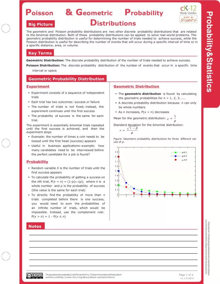
1. Poisson & Geometric Probability Probability&Statistics Study Guides Distributions Big Picture The geometric and Poisson probability distributions are two other discrete probability distributions that are related to the binomial distribution. Both of these probability distributions can be applied to solve real-world problems. The geometric probability distribution is useful for determining the number of trials needed to achieve success, while the Poisson distribution is useful for describing the number of events that will occur during a specific interval of time or in a specific distance, area, or volume. Key Terms Geometric Distribution: The discrete probability distribution of the number of trials needed to achieve success. Poisson Distribution: The discrete probability distribution of the number of events that occur in a specific time interval or space. Geometric Probability Distribution Experiment Geometric Distribution • Experiment consists of a sequence of independent • The geometric distribution is found by calculating trials the geometric probabilities for n = 1, 2, 3, .... • Each trial has two outcomes: success or failure • A discrete probability distribution because n can only • The number of trials is not fixed; instead, the be whole numbers experiment continues until the first success • As n increases, P(x = n) decreases • The probability of success is the same for each Mean for the geometric distribution: trial. Standard deviation for the binomial distribution: The experiment is essentially binomial trials repeated until the first success is achieved, and then the experiment stops • Example: the number of times a coin needs to be Figure: Geometric probability distributions for three different val- tossed until the first head (success) appears ues of p. • Useful in business applications–example: how many candidates need to be interviewed before the perfect candidate for a job is found? Probability • Random variable X is the number of trials until the first success appears • To calculate the probability of getting a success on the nth trial, P(x = n) = (1-p)n-1(p), where n is a whole number and p is the probability of success (this value is the same for each trial) • To directly find the probability of more than n trials completed before there is one success, you would need to sum the probabilities of an infinite number of trials, which would be impossible. Instead, use the complement rule: P(x > n) = 1 - P(x ≤ n) yourtextbookandisforclassroomorindividualuseonly. Disclaimer:thisstudyguidewasnotcreatedtoreplace Notes Page 1 of 2 ThisguidewascreatedbyLizhiFanandJinYu.Tolearnmoreaboutthestudent authors,visithttp://www.ck12.org/about/about-us/team/interns. v1.1.9.2012

2. Poisson & Geometric Probability Poisson Probability Distribution Distributions cont. Experiment Poisson Distribution • Experiment consists of counting the number of • The Poisson distribution is found by calculating the events that will occur during a specific interval Poisson probabilities for n = 1, 2, 3, .... of time or in a specific distance, area, or volume • A discrete probability distribution because n can only be • There are two outcomes: the event occurs whole numbers (success) or does not occur (failure) Mean for the geometric distribution: μ = λ • Each event is independent Probability • The probability that an event occurs during the Standard deviation for the binomial distribution: specified time interval or space is the same The experiment is a special case where the number of binomial trials gets larger and the probability of success gets smaller • Example: the number of traffic accidents at a particular intersection • Useful in predicting or estimating a number of things – planes at an airport, the number of fishes caught by a fisherman, arrival times, etc. Probability • Random variable X is the number of events that occur (successes) • To calculate the probability of n events, , where λ is the mean number of events in the time, distance, volume, or area Figure: Poisson probability distributions for three different values of •  e is approximately equal to 2.7183 λ. • To directly find the probability of more than For a binomial distribution where the number of trials n ≥ 100 events occuring, you would need to sum the and the probability of success p where np < 100, then the probabilities of an infinite number of trials, binomial distribution for k successes can be approximated which would be impossible. Instead, use the with a Poisson distribution where λ = np complement rule. Graphing Calculator In a graphing calculator, we can use built-in commands to find the geometric and Poisson distributions. Geometric Distribution The command for geometric distribution is: geometpdf(p, x). p is the probability of success, and x is the trial that we want the success to occur in. This will give us the probability of success occurring on that trial. There is another similar equation called geometcdf, which requires us to plug in two values for x: one low and one high. It will give us the probability of success occurring between those two trials. Poisson Distribution The command for Poisson distribution is: poissonpdf(λ, x). λ is the expected number of events, and x is the number of events. This will give us the probability that x many events occurred. There is a similar command called poissoncdf, which requires us to plug in two values for x: one low and one high. This will give us the probability the number of events that occurred fell between these two numbers. If you can’t find these commands, check the manual for your graphing calculator. For the TI-83/TI-84, both commands are found by pressing [2ND][DISTR]. Page 2 of 2