LECTURE 2-3. Course: “Design of Systems: Structural Approach” Dept. “Communication Networks &Systems”, Faculty of

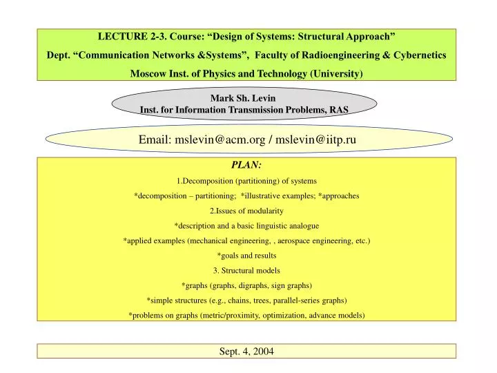
1. LECTURE 2-3. Course: “Design of Systems: Structural Approach” Dept. “Communication Networks &Systems”, Faculty of Radioengineering & Cybernetics Moscow Inst. of Physics and Technology (University) Mark Sh. Levin Inst. for Information Transmission Problems, RAS Email: mslevin@acm.org / mslevin@iitp.ru PLAN: 1.Decomposition (partitioning) of systems *decomposition – partitioning; *illustrative examples; *approaches 2.Issues of modularity *description and a basic linguistic analogue *applied examples (mechanical engineering, , aerospace engineering, etc.) *goals and results 3. Structural models *graphs (graphs, digraphs, sign graphs) *simple structures (e.g., chains, trees, parallel-series graphs) *problems on graphs (metric/proximity, optimization, advance models) Sept. 4, 2004

2. 1.Decomposition / partitioning of systems Decomposition: series process (e.g., dynamic programming) Partitioning: parallel process / dividing (combinatorial synthesis) Methods for partitioning: *physical partitioning *functional partitioning Examples (for airplane, for human) Examples for software: 1.Series information processing (input, solving, analysis, output) 2.Architecture: data subsystem, solving process, user interface, training subsystem, communication 3.Additional part: visualization (e.g., for data, for solving process) 4. Additional contemporary part (model management) as follows: *analysis of an initial applied situation, *library of models / methods, *selection / design of models / methods, *selection / design of multi-model solving strategy

3. 1.Decomposition / partitioning of systems: Example for multifunction system testing F1 F2 F3 Digraph of clusters Function clusters System functions Cluster F1 Cluster F2 Cluster F3

4. Main approaches to partitioning of systems A.Content analysis and experience: *by functions (basic functions, auxiliary functions) *by system parts (physical partitioning) B.Cluster analysis (clustering) Cluster F4 Cluster F2 Cluster F3 Cluster F5 Cluster F1 Cluster F6

5. 2.Issues of modularity PRINCIPLES FOR MANAGEMENT OF COMPLEXITY : *discrete pieces (modules) *standard interfaces for module communication Applications: *new technology design * organizational design LINGUISTIC SYSTEM TEXTS PRASES WORDS ABC

6. Applied examples for usage of modularity 1.Genetics 2.Reconfigurable manufacturing 3.Software libraries of standard modules 4.Combinatorial Chemistry: *molecular design in chemistry and biology *drug design *material engineering *etc. 5.Aerospace & mechanical engineering 6.Electronics 7.Civil engineering

7. Main goals of modularity and resume Main goals: 1.Management of complexity 2.Parallel work 3.Accomodation of future uncertainty 4.Variety of resultant modular systems 5.Flexibility, adaptability, reconfigurability of resultant modular systems Resume: 1.Simple design process & simple all phases of life cycle 2.Short life cycle of product, long life cycle of product modules 3.Reconfigurable systems (e.g., manufacturing systems): long life cycle for system generation 4.Simple design and support of product families (airplanes, cars, etc.) 5.Simple design and support of different products (on the basis of module libraries as reuse)

8. 3.Structural models A.GRAPHS 1.Graphs 2.Digraphs (directed graphs, oriented graphs - orgraphs) 3.Graphs / digraphs with weights (for vertices, for edges / arcs) 4.Simple graphs: chains, trees, parallel-series graphs, hierarchies 5.Sign graphs B.NETWORKS C.AUTOMATA D.BINARY RELATIONS

9. Illustration for graphs / digraphs Graph: G = (A,E) where a set of nodes (vertices) A={1,…,n} and a set of edges E A×A (pairs of nodes) Example: A={a, b, c}, E={(a, b), (b, c), (a, c)} a b c Matrix a b c a 1 1 b 1 1 c 1 1 Digraph (orgraph): G = (A,E) where a set of nodes (vertices) A={1,…,n} and a set of arcs E A×A (pairs of nodes) Example: A={a, b, c}, E={(a, a), (a, b), (b, c), (a, c)} a b c Matrix a b c a 1 1 1 b 1 c

10. Illustration for graphs with weights Graph (weights of edges): G = (A,E) where a set of nodes (vertices) A={1,…,n} and a set of edges E  A×A (pairs of nodes) Example: A={a, b, c}, E={(a, b), (b, c), (a, c)} a b c Matrix a b c a 2 5 b 2 3 c 5 3 Graph (weights of edges & nodes): G = (A,E) where a set of nodes (vertices) A={1,…,n} and a set of edges EA×A (pairs of nodes) Example: A={a, b, c}, E={(a, b), (b, c), (a, c)} (weights of nodes are pointed out in brackets) a(1) b(2) c(4) Matrix a b c a 2 5 b 2 3 c 5 3

11. Simple structures (chains, trees, parallel-series graphs) CHAIN TREE PARALLEL-SERIES GRAPH

12. Simple structures (hierarchy) Level 4 Level 3 Level 2 Level 1

13. Sign graph: illustrative examples - FOX Ecological system - + RABBIT + Manager Team a0 a0 - + + a1 a2 a1 a2 a3 a3 + + Engineer Technician Researcher -

14. Some advanced structural models 1.Multigraphs 2.Graphs with versions for nodes (vertices) 3.Graphs with “vector weights” 4.Graphs with fuzzy weights

15. Problems on graphs A.Metric / proximity (in graph between nodes, between graphs) Proximity between graphs: 1.metrics, 2.edit distance (minimal “cost” transformation), 3.common part B.Optimization on graphs: 1.Shortest path 2.Spanning tree (& close approximation problems: spanning by other simple structures) 3.Traveling salesman problem 4.Minimal Steiner tree 5.Ordering of vertices 6.Alocation on graphs 7.Covering problems C.Balance problem for sign graphs D.Clustering (dividing into interconnected groups)

16. Optimization problems on graphs: illustrations a5 a8 3 4 a1 a3 4 1 3 BASIC GRAPH (DIGRAPH): weights for arcs (or edges) 2 1 a9 a0 2 2 2 4 a4 a7 2 3 a6 a2 4 a5 a8 3 4 a1 a3 4 Shortest Path for < a0,a9 >: L = < a0,a1,a2,a3,a4,a7,a9 > 2+1+1+2+2 = 8 1 3 2 1 a9 a0 2 2 2 4 a4 a7 2 3 a6 a2 4

17. Optimization problems on graphs: illustrations Spanning tree (length = 19): a5 a8 a4 3 4 a1 a3 4 1 3 a3 a7 2 1 a9 a0 2 2 2 a1 4 a4 a9 a5 a6 a7 2 3 a6 a2 a0 a8 a2 4 Traveling Salesman Problem : L = < a0,a1,a3,a5,a7,a9,a8,a4,a2,a6> 2+1+3+4+2+2+3+4+4+4 a5 a8 3 4 a1 a3 4 1 3 2 1 a9 a0 2 2 2 4 a4 2 a7 3 a6 a2 4

18. Optimization problems on graphs: illustrations a5 a8 Steiner tree (example): a4 3 4 a1 a3 4 1 3 a3 a7 2 1 a9 a0 2 2 2 4 a4 a1 a7 a5 a6 2 3 a6 a2 4 a8 a0 a2 a9 “Ordering” Problem (close problems: sequencing, scheduling): a5 a8 3 4 a1 a0 a3 4 1 3 2 1 a9 a0 a1,a2,a3 2 2 2 4 a4 a4, a7 2 3 a6 a2 4 a5,a6,a7 a8,a9

19. Optimization problems on graphs: illustrations Allocation (assignment, mapping): Positions . . . Set of elements ALLOCATION (mapping, assignment)

20. Example: system function clusters and covering by chains (covering of arcs) Digraph of system function clusters F2 F1 F4 F3 F6 F5 F1 F2 F3 F4 F5 F6 F3 F1 F3 F5 F3

21. Illustration for clustering a5 a8 3 4 a1 a3 4 1 3 2 1 a9 a0 Basic graph 2 2 2 4 a4 2 a7 3 a6 a2 4 a5 a8 Clusters (a version): C1 = { a0 , a1 } C2 = { a3 , a5 } C3 = { a8 , a9 } C4 = { a2 , a4 , a6 , a7 } 3 a1 a3 3 2 a0 a9 2 4 a4 a7 3 a6 a2 4

22. Binary relations Initial set A = {1, 2, …, n}, B = A × A (  (x, y) such that x, y A) Definition. Binary relation R is a subset of B EXAMPLE: A={a, b, c, d} B = {(a, a), (a, b), (a, c), (a, d), (b, a), (b, a), (b, c), (b, d), (c, a), (c, b), (c, c), (c, d), (d, a), (d, b), (d, c), (d, d)} R1 = { (a, b), (b, c), (c, b), (d, c) } R2 = { (a, d), (b, d), (a, c) } R3 =R1& R2 a b a b a b R1 R2 R3=R1&R2 d c d d c c

23. Binary relations Context Examples: 1.”Better” (dominance) 2.”Better & Equal” (dominance & equivalence) 3.”Equal” (equivalence) SOME PROPERTIES: 1.Symmetry: (x, y)  R => (y, x)  R ( x  R, y  R) 2.Reflexivity: (x, x)  R x  R 3.Transitivity: (x, y)  R , (y, z)  R =>(x, z)  R ( x  R, y  R , z  R) APPLICATIONS: *Friendship, *Partnership, *Similarity, *Etc. Extended models: 1.Weighted binary relations (e.g., power of dominance) 2.K-relations Prospective usage: Combinatorial optimization problems on graphs with additional binary relations (over node/vertices, over edges / arcs, over elements / positions)