Download
1 / 60
950 likes | 2.22k Vues
Nanomaterials. Nathan Liang Paul Maynard Wei Li . Nanotechnology. What is Nanotechnology?. It comprises any technological developments on the nanometer scale, usually 0.1 to 100 nm. One nanometer equals one thousandth of a micrometer or one millionth of a millimeter.

E N D
Nanomaterials Nathan Liang Paul Maynard Wei Li
What is Nanotechnology? • It comprises any technological developments on the nanometer scale, usually 0.1 to 100 nm. • One nanometer equals one thousandth of a micrometer or one millionth of a millimeter. • It is also referred as microscopic technology.
Molecular Nanotechnology • The term nanotechnology is often used interchangeably with molecular nanotechnology (MNT) • MNT includes the concept of mechanosynthesis. • MNT is a technology based on positionally-controlled mechanosynthesis guided by molecular machine systems.
Nanotechnologyin Field of Electronics • Miniaturization • Device Density
History • Richard Feynman • 1959, entitled ‘There's Plenty of Room at the Bottom’ • Manipulate atoms and molecules directly • 1/10th scale machine to help to develop the next generation of 1/100th scale machine, and so forth. • As things get smaller, gravity would become less important, surface tension molecule attraction would become more important.
History • Tokyo Science University professor Norio Taniguchi • 1974 to describe the precision manufacture of materials with nanometre tolerances. • K Eric Drexler • 1980s the term was reinvented • 1986 book Engines of Creation: The Coming Era of Nanotechnology. • He expanded the term into Nanosystems: Molecular Machinery, Manufacturing, and Computation
Nanomaterial and Devices • Small Scales • Extreme Properties • Nanobots
Self-Assemble • Nanodevices build themselves from the bottom up. • Scanning probe microscopy • Atomic force microscopes • scanning tunneling microscopes • scanning the probe over the surface and measuring the current, one can thus reconstruct the surface structure of the material
Problems in Nanotechnology • how to assemble atoms and molecules into smart materials and working devices? • Supramolecular chemistry • self-assemble into larger structures
Current Nanotechnology • Stanford University • extremely small transistor • two nanometers wide and regulates electric current through a channel that is just one to three nanometers long • ultra-low-power
Intel • processors with features measuring 65 nanometers Gate oxide less than 3 atomic layers thick 20 nanometer transistor Atomic structure
Plasmons • Waves of electrons traveling along the surface of metals • They have the same frequency and electromagnetic field as light. • Their sub-wavelength require less space. • With the use of plasmons information can be transferred through chips at an incredible speed
What I will cover • Carbon Nanotubes • Bio-Nano-Materials • Thermoelectric Nanomaterials • What is happening at UK
Carbon Nanotubes • What are they? • Carbon molecules aligned in cylinder formation • Who discovered them? • Researchers at NEC in 1991 • What are some of their uses? • Minuscule wires • Extremely small devices
Potential energy • Vk = Repulsive force • Va = attractive force • Morse potential equations
Carbon Nanotubes • total potential of a system • Adds the NB contribution • Force of interaction
Carbon Nanotubes • Leonard – Jones potential with von der Waals interaction • Geen - Kudo relation
Bio-Nanomaterials • What is Bio-Nanomaterials? • Putting DNA inside of carbon nanotubes • What can this research give us? • There are lots of chemical and biological applications
Thermoelectric Nanomaterials Concepts before modeling can begin: • ZT = TσS2/κ • T = temperature • σ = electrical conductivity • S = Seebeck constant • κ = κph +κel • K = sum of lattice and electronic contributions • Potential across thermoelectric material • Boltzmann transport
Nanomaterials at UK • Deformation Mechanisms of Nanostructured Materials • Synthesis of Nanoporous Ceramics by Engineered Molecular Assembly • Carbon Nanotubes • Optical-based Nano-Manufacturing • The Grand Quest: CMOS High-k Gate Insulators • Self-assembled metal alloy nanostructures • Rare-earth Monosulfides: From Bulk Samples to Nanowires • Thermionic Emission and Energy Conversion with Quantum Wires • Resonance-Coupled Photoconductive Decay
1. Davis, H. T., Bodet, J. F., Scriven, L. E., Miller, W. G. Physics of Amphiphilic Layers, 1987, Springer-Verlag, New York Introduction to surfactant and self-assembly • What is surfactant? • What is self-assembly? • Micelles, mesophases
Introduction to fluorinated surfactants • Unique properties introduced by the strong electronegativity of fluorine and the efficient shielding of the carbon atoms by fluorine atoms • Fluorocarbon chain is stiffer, and favors aggregates with low curvature (Fig from [2]) • Advantages over hydrocarbon chains: higher surface activity , thermal, chemical, and biological inertness, gas dissolving capacity, higher hydrophobicityand lipophobicity 2. M. Sprik, U. Rothlisberger and M. L. Klein, Molec. Phys.1999 97:3553. K. Wang, G. Karlsson, M. Almgren and T. Asakawa, J. Phys. Chem. B1999 103:92374. E. Fisicaro, A. Ghiozzi, E. Pelizzetti, G. Viscardi and P. L. Quagliotto, J. Coll. Int. Sci.1996 182:549
Motivations for the computer simulation of fluorinated surfactants • Simulations can be treated as computer experiments that serve as adjuncts to theory and real experiments • Experiment is a viable way to study the effect of chain stiffness, yet it might be expensive to do a systematic study on this topic. • Computer simulations might help selecting surfactants for the right type of mesophase, which provides a guideline for experimental study.
Monte Carlo techniques for the simulation of surfactant solutions • Off-lattice atomistic simulation • All atoms (or small group of atoms, e.g. CH2) are explicitly represented • Most interactions are included, more realistic, yet hard to model • Can simulates molecular trajectories on a time-scale of nanoseconds • Can’t simulation the self-assembly phenomena • Off-lattice coarse-grain • A number of atoms are grouped together and represented in a simplified manner • Electrostatic and dihedral angle potentials are usually absent • Can simulate process happening on a time-scale of microseconds, e.g. micelle formation • Can’t simulate equilibrium self-assembly structure at higher concentration
Monte Carlo techniques for the simulation of surfactant solutions (continued) • Lattice coarse-grain • replacing the continuous space with a discretized lattice of suitable geometry • Electrostatic and intra-molecular potentials are absent • Fast, efficient, can simulate process happening on a time-scale of a few hours, e.g. mesophase formation • Based on Flory-Huggins Theory. Proven to be successful in polymer science for many years for investigating universal properties of single chains, polymer layers and solutions and melts • Utility of the model is limited
Choosing the right model for our simulation purpose – lattice coarse-grain • Most time-consuming part in a MC simulation is the evaluation of inter and intra-molecular potentials after each trial move • The speed of off-lattice models is limited, because • It has to reevaluate the potential functions explicitly when calculate the energy change after each move • The speed of the simulation is determined by the complexity of the potential functions • Off-lattice can at most simulate the formation of a few micelles • Lattice models are fast, because • Atoms (united atoms) are moving on the lattice, intra and inter-molecular distance, bond angles are thus discretized • It’s possible to precalculate the potentials corresponding to certain distance and angles and build look-up tables • When calculate the energy change, only need to look up the tables • Can simulate the mesophase formation efficiently • Our targeted system: mesophase formation in surfactant solutions
Larson’s Lattice Model – representation of the system • Targeted system: a surfactant solution consists of NA moles water, NB moles oil and Nc moles surfactant molecules, with fixed volume and temperature (canonical ensemble) • Surfactant: use HiTj to define a linear surfactant consisting of a string of consecutive i head units attached to consecutive j tail units. • Whole system resides on an N×N×N cubic lattice, periodic boundary conditions are applied • Oil and water molecules occupy single sites on the lattice, and each amphiphile occupies a sequence of adjacent or diagonally adjacent sites (equal molar volume for all the species) • Number of sites occupied by surfactant is, • The rest of the sites is fully occupied by water and oil according to their volume ratio
Square-well potential A simple 2D lattice with 2 chains, 7 water (grey) and 6 oil (red) molecules (i, j=water, oil, head, tail) Larson’s Lattice Model – interactions between species • Each site interacts only with its 8 nearest, 9 diagonally nearest, and 9 body-diagonally nearest neighbors • Essentially, a square well potential is applied • Favorable interactions are set to be -1, while unfavorable interactions are +1 • Total energy is pairwise additive
Larson’s Lattice Model - typical trial moves • Pair interchange [5] • Exchange of positions of two simple molecules • Chain kink [5] • A surfactant segment exchanges position with its neighbor without breaking the surfactant chain • Chain reptation [5] • One chain end moves to a neighboring site, and the rest of that chain slithers a unit to keep the chain connectivity • Chain multiple kink [6] • If a kink move creates a single break in the chain, the simple molecule will continue to exchange with subsequent beads along the chain until beads on the chain are close enough to reconnect. 5. R. G. Larson, L.E. Scriven and H. T. Davis, J. Chem. Phys. ,1985, 83, 2411 6. K.R. Haire, T.J. Carver, A.H. Windle, Computational and Theoretical Polymer Science, 2001, 11, 17
A simple 2D lattice with 2 chains, 7 water (grey) and 6 oil (red) molecules Larson’s Lattice Model – simulation process • Initialize the system • Put the system in a random state • Make a trial move • Randomly conduct a trial move according toits occurrence ratio • Calculate the energy change • Reevaluate the interactions of the moved particles with its neighbors and calculate the energy change • Accept the trial move with the Metropolis scheme • Keep trying the moves until system approach equilibrium • Either monitor the total energy change, or monitor the structure formed in the simulation box • Sampling • Sample a certain property over a certain number of configurations
Simulation of the mesophase formation - preliminary results • Simulation procedure: • Start the simulation from a higher temperature and equilibrate the system, in order to make the system in a athermal state and as random as possible • Anneal the system by decreasing the temperature in a small amount after the system reaches equilibrium at a higher temperature • When the temperature is lower than the critical temperature, sample the density of a certain species • Preliminary results • 60vol% H4T4 surfactant, 40vol% water • Should form cylindrical structure according to Larson’s report [7] • The right figures are the same self-assembly structure viewed from two different perspectives 3D density contour plot according to the oil concentration. 60% H4T4 surfactant, 40% water 7. R. G. Larson; Chemical Engineering Science, 1994, 49, 17, 2833
Add the bond overlapping constraint • Bond overlapping may occurred in the system, which is unrealistic • Simulation results after adding the bond overlapping constrain (other conditions are the same). Perfect hexagonal close packing cylindrical structure is formed. Two chains overlaps with each other 3D density contour plot according to the oil concentration. 60% H4T4 surfactant, 40% water
Verification of our lattice simulation program – compare with Larson’s simulation results • Ternary phase diagram of H4T4 surfactant in water and oil by Larson’s lattice Monte Carlo simulation [8] • 5 data points (volume percentage) • 40% water, 40% oil, 20% surfactant • 20% water, 40% oil, 40% surfactant • 20% water, 45% oil, 35% surfactant • 60% water, 40% surfactant • 7.3% water, 32.7% oil, 60% surfactant • 40% water, 60% surfactant 8. R. G. Larson; J. Phys. II France, 1996, 6, 1441
Simulation results from our simulation program • 40% water, 40% oil, 20% surfactant - Bicontinuous mesophase • 20% water, 40% oil, 40% surfactant - lamellar without holes mesophase • 20% water, 45% oil, 35% surfactant - lamellar with holes mesophase Left: oil concentration profile, Right: water concentration profile