Download
1 / 57
570 likes | 1.06k Vues
ASSUMPTION C.7. Assumptions for Model C C.7 The disturbance term is distributed independently of the regressors u t is distributed independently of X jt' for all t' (including t ) and j (1) The disturbance term in any observation is distributed independently of the values of the

E N D
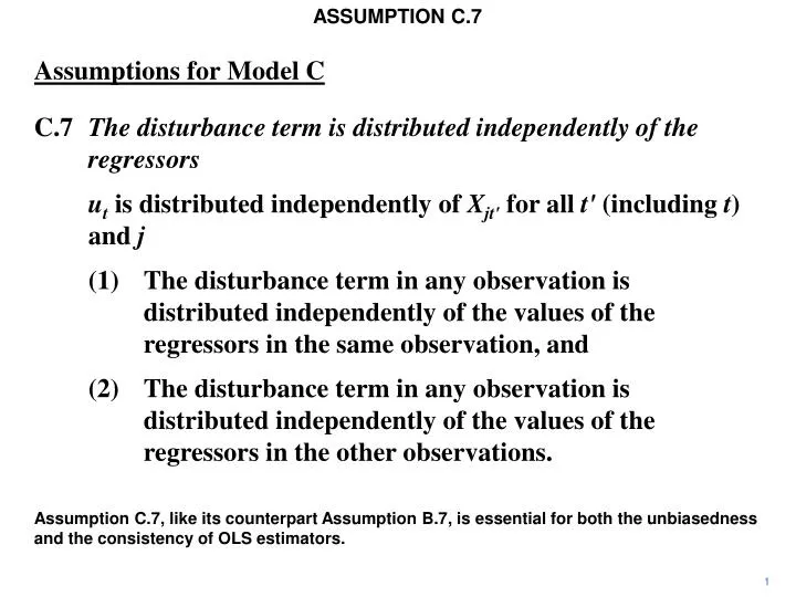
ASSUMPTION C.7 Assumptions for Model C C.7 The disturbance term is distributed independently of the regressors ut is distributed independently of Xjt' for all t' (including t) and j (1) The disturbance term in any observation is distributed independently of the values of the regressors in the same observation, and (2) The disturbance term in any observation is distributed independently of the values of the regressors in the other observations. Assumption C.7, like its counterpart Assumption B.7, is essential for both the unbiasedness and the consistency of OLS estimators. 1
ASSUMPTION C.7 Assumptions for Model C C.7 The disturbance term is distributed independently of the regressors ut is distributed independently of Xjt' for all t' (including t) and j (1) The disturbance term in any observation is distributed independently of the values of the regressors in the same observation, and (2) The disturbance term in any observation is distributed independently of the values of the regressors in the other observations. It is helpful to divide it into two parts, as shown above. Both parts are required for unbiasedness. However only the first part is required for consistency (as a necessary, but not sufficient, condition). 2
ASSUMPTION C.7 Assumptions for Model C C.7 The disturbance term is distributed independently of the regressors ut is distributed independently of Xjt' for all t' (including t) and j (1) The disturbance term in any observation is distributed independently of the values of the regressors in the same observation, and (2) The disturbance term in any observation is distributed independently of the values of the regressors in the other observations. For cross-sectional regressions, Part (2) is rarely an issue. Since the observations are generated randomly there is seldom any reason to suppose that the disturbance term in one observation is not independent of the values of the regressors in the other observations. 3
ASSUMPTION C.7 Assumptions for Model C C.7 The disturbance term is distributed independently of the regressors ut is distributed independently of Xjt' for all t' (including t) and j (1) The disturbance term in any observation is distributed independently of the values of the regressors in the same observation, and (2) The disturbance term in any observation is distributed independently of the values of the regressors in the other observations. Hence unbiasedness really depended on part (1). Of course, this might fail, as we saw with measurement errors in the regressors and with simultaneous equations estimation. 4
ASSUMPTION C.7 Assumptions for Model C C.7 The disturbance term is distributed independently of the regressors ut is distributed independently of Xjt' for all t' (including t) and j (1) The disturbance term in any observation is distributed independently of the values of the regressors in the same observation, and (2) The disturbance term in any observation is distributed independently of the values of the regressors in the other observations. With time series regression, part (2) becomes a major concern. To see why, we will review the proof of the unbiasedness of the OLS estimator of the slope coefficient in a simple regression model. 5
ASSUMPTION C.7 The slope coefficient may be written as shown above. 6
ASSUMPTION C.7 We substitute for Y from the true model. 7
ASSUMPTION C.7 The b1 terms in the second factor in the numerator cancel each other. Rearranging what is left, we obtain the third line. 8
ASSUMPTION C.7 The first term in the numerator, when divided by the denominator, reduces to b2. Hence as usual we have decomposed the slope coefficient into the true value and an error term. 9
ASSUMPTION C.7 The error term can be decomposed as shown. 10
ASSUMPTION C.7 – u is a common factor in the second component of the error term and so can be brought out of it as shown. 11
ASSUMPTION C.7 It can then be seen that the numerator of the second component of the error term is zero. 12
ASSUMPTION C.7 We are thus able to show that the OLS slope coefficient can be decomposed into the true value and an error term that is a weighted sum of the values of the disturbance term in the observations, with weights ai defined as shown. 13
ASSUMPTION C.7 Now we will take expectations. The expectation of the right side of the equation is the sum of the expectations of the individual terms. 14
ASSUMPTION C.7 If the ui are distributed independently of the ai, we can decompose the E(aiui) terms as shown. 15
ASSUMPTION C.7 Unbiasedness then follows from the assumption that the expectation of ui is zero. 16
ASSUMPTION C.7 The crucial step is the previous one, which requires ui to be distributed independently of ai. ai is a function of all of the X values in the sample, not just Xi. So Part (1) of Assumption C.7, that ui is distributed independently of Xi, is not enough. 17
ASSUMPTION C.7 We also need Part (2), that ui is distributed independently of Xj, for all j. 18
ASSUMPTION C.7 In regressions with cross-sectional data this is usually not a problem. 19
ASSUMPTION C.7 Cross-sectional data: LGEARNi = b1 + b2Si + ui LGEARNj = b1 + b2Sj + uj Reasonable to assume uj and Si independent (i≠ j). The main issue is whether ui is independent of Si. If, for example, we are relating the logarithm of earnings to schooling using a sample of individuals, it is reasonable to suppose that the disturbance term affecting individual I will be unrelated to the schooling of any other individual. 20
ASSUMPTION C.7 Cross-sectional data: LGEARNi = b1 + b2Si + ui LGEARNj = b1 + b2Sj + uj Reasonable to assume uj and Si independent (i≠ j). The main issue is whether ui is independent of Si. Assuming this, the independence of ui and ai then depends only on the independence of ui and Si. 21
ASSUMPTION C.7 Time series data: Yt = b1 + b2Yt–1 + ut Yt+1 = b1 + b2Yt + ut+1 The disturbance term ut is automatically correlated with the explanatory variable Yt in the next observation. However with time series data it is different. Suppose, for example, that you have a model with a lagged dependent variable as a regressor. Here we have a very simple model where the only regressor is the lagged dependent variable. 22
ASSUMPTION C.7 Time series data: Yt = b1 + b2Yt–1 + ut Yt+1 = b1 + b2Yt + ut+1 The disturbance term ut is automatically correlated with the explanatory variable Yt in the next observation. We will suppose that Part (1) of Assumption C.7 is valid and that ut is distributed independently of Yt–1. 23
ASSUMPTION C.7 Time series data: Yt = b1 + b2Yt–1 + ut Yt+1 = b1 + b2Yt + ut+1 The disturbance term ut is automatically correlated with the explanatory variable Yt in the next observation. Even if Part (1) is valid, Part (2) must be invalid in this model. 24
ASSUMPTION C.7 Time series data: Yt = b1 + b2Yt–1 + ut Yt+1 = b1 + b2Yt + ut+1 The disturbance term ut is automatically correlated with the explanatory variable Yt in the next observation. ut is a determinant of Yt and Yt is the regressor in the next observation. Hence even if ut is uncorrelated with the explanatory variable Yt–1 in the observation for Yt, it will be correlated with the explanatory variable Yt in the observation for Yt+1. 25
ASSUMPTION C.7 Time series data: Yt = b1 + b2Yt–1 + ut Yt+1 = b1 + b2Yt + ut+1 The disturbance term ut is automatically correlated with the explanatory variable Yt in the next observation. X As a consequence ui is not independent of ai and so we cannot write E(aiui) = E(ai)E(ui). It follows that the OLS slope coefficient will in general be biased. 26
ASSUMPTION C.7 Time series data: Yt = b1 + b2Yt–1 + ut Yt+1 = b1 + b2Yt + ut+1 The disturbance term ut is automatically correlated with the explanatory variable Yt in the next observation. X We cannot obtain a closed-form analytical expression for the bias. However we can investigate it with Monte Carlo simulation. 27
ASSUMPTION C.7 Yt = 10 + 0.8Yt–1 + ut n = 20 n = 1000 Sample b1 s.e.(b1) b2 s.e.(b2)b1s.e.(b1)b2 s.e.(b2) 1 24.3 10.2 0.52 0.20 11.0 1.0 0.78 0.02 2 12.6 8.1 0.74 0.16 11.8 1.0 0.76 0.02 3 26.5 11.5 0.49 0.22 10.8 1.0 0.78 0.02 4 28.8 9.3 0.43 0.18 9.4 0.9 0.81 0.02 5 10.5 5.4 0.78 0.11 12.2 1.0 0.76 0.02 6 9.5 7.0 0.81 0.14 10.5 1.0 0.79 0.02 7 4.9 7.4 0.91 0.15 10.6 1.0 0.79 0.02 8 26.9 10.5 0.47 0.20 10.3 1.0 0.79 0.02 9 25.1 10.6 0.49 0.22 10.0 0.9 0.80 0.02 10 20.9 8.8 0.58 0.18 9.6 0.9 0.81 0.02 We will start with the very simple model shown at the top of the slide. Y is determined only by its lagged value, with intercept 10 and slope coefficient 0.8. 28
ASSUMPTION C.7 Yt = 10 + 0.8Yt–1 + ut n = 20 n = 1000 Sample b1 s.e.(b1) b2 s.e.(b2)b1s.e.(b1)b2 s.e.(b2) 1 24.3 10.2 0.52 0.20 11.0 1.0 0.78 0.02 2 12.6 8.1 0.74 0.16 11.8 1.0 0.76 0.02 3 26.5 11.5 0.49 0.22 10.8 1.0 0.78 0.02 4 28.8 9.3 0.43 0.18 9.4 0.9 0.81 0.02 5 10.5 5.4 0.78 0.11 12.2 1.0 0.76 0.02 6 9.5 7.0 0.81 0.14 10.5 1.0 0.79 0.02 7 4.9 7.4 0.91 0.15 10.6 1.0 0.79 0.02 8 26.9 10.5 0.47 0.20 10.3 1.0 0.79 0.02 9 25.1 10.6 0.49 0.22 10.0 0.9 0.80 0.02 10 20.9 8.8 0.58 0.18 9.6 0.9 0.81 0.02 The disturbance term u will be generated using random numbers drawn from a normal distribution with mean 0 and variance 1. The sample size is 20. 29
ASSUMPTION C.7 Yt = 10 + 0.8Yt–1 + ut n = 20 n = 1000 Sample b1 s.e.(b1) b2 s.e.(b2)b1s.e.(b1)b2 s.e.(b2) 1 24.3 10.2 0.52 0.20 11.0 1.0 0.78 0.02 2 12.6 8.1 0.74 0.16 11.8 1.0 0.76 0.02 3 26.5 11.5 0.49 0.22 10.8 1.0 0.78 0.02 4 28.8 9.3 0.43 0.18 9.4 0.9 0.81 0.02 5 10.5 5.4 0.78 0.11 12.2 1.0 0.76 0.02 6 9.5 7.0 0.81 0.14 10.5 1.0 0.79 0.02 7 4.9 7.4 0.91 0.15 10.6 1.0 0.79 0.02 8 26.9 10.5 0.47 0.20 10.3 1.0 0.79 0.02 9 25.1 10.6 0.49 0.22 10.0 0.9 0.80 0.02 10 20.9 8.8 0.58 0.18 9.6 0.9 0.81 0.02 Here are the estimates of the coefficients and their standard errors for 10 samples. We will start by looking at the distribution of the estimate of the slope coefficient. 8 of the estimates are below the true value and only 2 above. 30
ASSUMPTION C.7 Yt = 10 + 0.8Yt–1 + ut n = 20 n = 1000 Sample b1 s.e.(b1) b2 s.e.(b2)b1s.e.(b1)b2 s.e.(b2) 1 24.3 10.2 0.52 0.20 11.0 1.0 0.78 0.02 2 12.6 8.1 0.74 0.16 11.8 1.0 0.76 0.02 3 26.5 11.5 0.49 0.22 10.8 1.0 0.78 0.02 4 28.8 9.3 0.43 0.18 9.4 0.9 0.81 0.02 5 10.5 5.4 0.78 0.11 12.2 1.0 0.76 0.02 6 9.5 7.0 0.81 0.14 10.5 1.0 0.79 0.02 7 4.9 7.4 0.91 0.15 10.6 1.0 0.79 0.02 8 26.9 10.5 0.47 0.20 10.3 1.0 0.79 0.02 9 25.1 10.6 0.49 0.22 10.0 0.9 0.80 0.02 10 20.9 8.8 0.58 0.18 9.6 0.9 0.81 0.02 This suggests that the estimator is downwards biased. However it is not conclusive proof because an 8–2 split will occur quite frequently even if the estimator is unbiased. (If you are good at binomial distributions, you will be able to show that it will occur 11% of the time.) 31
ASSUMPTION C.7 Yt = 10 + 0.8Yt–1 + ut n = 20 n = 1000 Sample b1 s.e.(b1) b2 s.e.(b2)b1s.e.(b1)b2 s.e.(b2) 1 24.3 10.2 0.52 0.20 11.0 1.0 0.78 0.02 2 12.6 8.1 0.74 0.16 11.8 1.0 0.76 0.02 3 26.5 11.5 0.49 0.22 10.8 1.0 0.78 0.02 4 28.8 9.3 0.43 0.18 9.4 0.9 0.81 0.02 5 10.5 5.4 0.78 0.11 12.2 1.0 0.76 0.02 6 9.5 7.0 0.81 0.14 10.5 1.0 0.79 0.02 7 4.9 7.4 0.91 0.15 10.6 1.0 0.79 0.02 8 26.9 10.5 0.47 0.20 10.3 1.0 0.79 0.02 9 25.1 10.6 0.49 0.22 10.0 0.9 0.80 0.02 10 20.9 8.8 0.58 0.18 9.6 0.9 0.81 0.02 However the suspicion of a bias is reinforced by the fact that many of the estimates below the true value are much further from it than those above. The mean value of the estimates is 0.62. 32
ASSUMPTION C.7 Yt = 10 + 0.8Yt–1 + ut n = 20 n = 1000 Sample b1 s.e.(b1) b2 s.e.(b2)b1s.e.(b1)b2 s.e.(b2) 1 24.3 10.2 0.52 0.20 11.0 1.0 0.78 0.02 2 12.6 8.1 0.74 0.16 11.8 1.0 0.76 0.02 3 26.5 11.5 0.49 0.22 10.8 1.0 0.78 0.02 4 28.8 9.3 0.43 0.18 9.4 0.9 0.81 0.02 5 10.5 5.4 0.78 0.11 12.2 1.0 0.76 0.02 6 9.5 7.0 0.81 0.14 10.5 1.0 0.79 0.02 7 4.9 7.4 0.91 0.15 10.6 1.0 0.79 0.02 8 26.9 10.5 0.47 0.20 10.3 1.0 0.79 0.02 9 25.1 10.6 0.49 0.22 10.0 0.9 0.80 0.02 10 20.9 8.8 0.58 0.18 9.6 0.9 0.81 0.02 To determine whether the estimator is biased or not, we need a greater number of samples. 33
ASSUMPTION C.7 Yt = 10 + 0.8Yt–1 + ut mean = 0.6233 (n = 20) 0.8 The chart shows the distribution with 1 million samples. This settles the issue. The estimator is biased downwards. 34
ASSUMPTION C.7 Yt = 10 + 0.8Yt–1 + ut mean = 0.6233 (n = 20) 0.8 There is a further puzzle. If the disturbance terms are drawn randomly from a normal distribution, as was the case in this simulation, and the regression model assumptions are valid, the regression coefficients should also have normal distributions. 35
ASSUMPTION C.7 Yt = 10 + 0.8Yt–1 + ut mean = 0.6233 (n = 20) 0.8 However the distribution is not normal. It is negatively skewed. 36
ASSUMPTION C.7 Yt = 10 + 0.8Yt–1 + ut mean = 0.6233 (n = 20) 0.8 Nevertheless the estimator may be consistent, provided that certain conditions are satisfied. 37
ASSUMPTION C.7 Yt = 10 + 0.8Yt–1 + ut mean = 0.7650 (n = 100) mean = 0.6233 (n = 20) 0.8 When we increase the sample size from 20 to 100, the bias is much smaller. (X has been assigned the values 1, …, 100. The distribution here and for all the following diagrams is for 1 million samples.) 38
ASSUMPTION C.7 Yt = 10 + 0.8Yt–1 + ut mean = 0.7966 (n = 1000) mean = 0.7650 (n = 100) mean = 0.6233 (n = 20) 0.8 If we increase the sample size to 1,000, the bias almost vanishes. (X has been assigned the values 1, …, 1,000.) 39
ASSUMPTION C.7 Yt = 10 + 0.5Xt + 0.8Yt–1 + ut mean = 0.4979 (n = 20) mean = 1.2553 (n = 20) 0.8 Here is a slightly more realistic model with an explanatory variable Xt as well as the lagged dependent variable. 40
ASSUMPTION C.7 Yt = 10 + 0.5Xt + 0.8Yt–1 + ut mean = 0.4979 (n = 20) mean = 1.2553 (n = 20) 0.8 The estimate of the coefficient of Yt–1 is again biased downwards, more severely than before (black curve). The coefficient of Xt is biased upwards (red curve). 41
ASSUMPTION C.7 Yt = 10 + 0.5Xt + 0.8Yt–1 + ut mean = 0.7441 (n = 100) mean = 0.6398 (n = 100) mean = 1.2553 (n = 20) mean = 0.4979 (n = 20) 0.8 If we increase the sample size to 100, the coefficients are much less biased. 42
ASSUMPTION C.7 Yt = 10 + 0.5Xt + 0.8Yt–1 + ut mean = 0.7947 (n = 1000) mean = 0.5132 (n = 1000) 0.8 If we increase the sample size to 1,000, the bias almost disappears, as in the previous example. 43
ASSUMPTION C.7 In both of these examples the OLS estimators were consistent, despite being biased for finite samples. We will explain this for the first example. The slope coefficient can be decomposed as shown in the usual way. 44
ASSUMPTION C.7 We will show that the plim of the error term is 0. As it stands, neither the numerator nor the denominator possess limits, so we cannot invoke the plim quotient rule. 45
ASSUMPTION C.7 We divide the numerator and the denominator by n. 46
ASSUMPTION C.7 Now we can invoke the plim quotient rule, because it can be shown that the plim of the numerator is the covariance of Yt–1 and ut and the plim of the denominator is the variance of Yt–1. 47
ASSUMPTION C.7 If Part (1) of Assumption C.7 is valid, the covariance between ut and Yt–1 is zero. In this model it is reasonable to suppose that Part(1) is valid because Yt–1 is determined before ut is generated. 48
ASSUMPTION C.7 Thus the plim of the slope coefficient is equal to the true value and the slope coefficient is consistent. 49
ASSUMPTION C.7 You will often see models with lagged dependent variables in the applied literature. Usually the problem discussed in this slideshow is ignored. This is acceptable if the sample size is large enough, but if the sample is small, there is a risk of serious bias. 50