Download

1 / 61
610 likes | 978 Vues
I. International Capital Mobility a. Why international capital flows ? (i) Capital flows as a counterpart of the exchange of goods (see point b) Trade balance = Net capital outflows Exchange of goods results from differences across countries: productivity, endowments, time preference.

E N D
(i) Capital flows as a counterpart of the exchange of goods (see point b) • Trade balance = Net capital outflows • Exchange of goods results from differences across countries: productivity, endowments, time preference.
(ii) Capital flows as exchange of assets to hedge risks • Risks result from changes in prices - raw materials: gold, oil… - exchange rate: relative price of one good between two countries - assets
Example €/$ • Imagine a US computer maker firm (A) and a European distribution firm (B). • B places an order with A of 300 computers in 02/04. A will deliver these 300 computers with a delay in 05/04. • Computer’s Price: 1000USD • 02/04: 1€->1.25 USD • 05/04: 1€->1.2 USD
B has to pay in USD so he will support this exchange rate risk. • If B pays when it orders in 02/04, the cost will be 240 000€ • If B pays at the delivery in 05/04, the cost will be 250 000€ • The spread between those payments (10 000 €) reflects changes in USD/€ exchange rate. • B can ask the bank to hedge this foreign exchange risk. Otherwise, changes in exchange rates will be supported by the buyers of B’s computers.
These risks are more present because of higher capital mobility. • There is a risk when prices fluctuate. • Risk on exchange rates were reduced in the Bretton Woods system.
Hedge’s instruments (see Mishkin, Chapter 13) • Financial derivatives are used to eliminate the price risk inherent in transactions that call for future delivery of money, a security, or a commodity. • Buying an asset is taking a long position. • Selling an asset for a future delivery is taking a short position. • Principle’s of hedging is to offset a long position by taking an additional short position or offset a short position by taking an additional long position.
Hedge’s instruments • Forward contracts are agreements by two parties to engage in a financial transaction at a future point in time. • Futures contract are traded on organized exchanges such as the Montreal Exchange in Canada. • Futures contracts are standardized (↑size of the market -> ↑ liquidity) and parties are engaged with an intermediate (the clearinghouse) to prevent from the risk of default.
Example • B has to buy USD in 2 months. • He has to enter in a forward contract: he will engage now to buy in 2 months 300 000 USD against 240 000 € at the current exchange rate (1€->1.25USD). • Otherwise B could address to the Chicago Mercantile Exchange for a euro contract delivered in May. The amount is 1000€ by contract with an exchange rate of 1.25USD. So B needs 240 contracts to sell 240 000€ in May against 300 000 USD.
Hedge’s instruments • Options are contracts that give the purchaser the right to buy or sell the underlying financial instrument at a specified price (exercise price) within a specific period of time. • The writer (seller) of the option is forced to buy or sell the financial instrument to the owner (buyer) but the owner does not have to exercise the option.
Hedge’s instruments • A call option is a contract that gives the owner the right to buy a financial instrument at the exercise price within a specific period of time. • A put option is a contract that gives the owner the right to sell a financial instrument at the exercise price within a specific period of time.
Example • 02/04 : 1€->1.25USD • Imagine that 05/04 the €/USD has appreciated (1€->1.3 USD) then B loses with a forward contract but not with an option because in this case he will not exercise the option.
b. The reasons of exchange (i) Static analysis: some aspects of international trade (differences in productivity, in endowments) (ii) Dynamic analysis: intertemporal choice
(i) Static analysis • We assume here that trade balance is always zero so that there are no capital flows. • International trade exists because countries are different (productivity, factors endowment) • Trade implies price convergence • To study the effects of trade, we distinguish: • An autarky economy (AE) • A trading economy (TE) -> Countries have an advantage to exchange when there exists a gap between prices in the AE and the TE.
This section: -> why countries benefit from international trade? ->what are the consequences of international trade on prices? • Same answer around three different international trade models: -> Because countries are different -> International trade leads to a price convergence (i-a) the Ricardian model (i-b) the Factor Specific model (i-c) the Hecksher Olhin model
(i-a) The Ricardian Model • Introduction • The Concept of Comparative Advantage • A One-Factor Economy • Trade in a One-Factor World
Introduction • Countries engage in international trade for two basic reasons: • They are different from each other in terms of climate, land, capital, labor, and technology. • They try to achieve scale economies in production. • The Ricardian model is based on technological differences across countries. • These technological differences are reflected in differences in the productivity of labor.
The Concept of Comparative Advantage • If each country exports the goods in which it has comparative advantage (lower opportunity costs), then all countries can in principle gain from trade. • What determines comparative advantage? • Answering this question would help us understand how country differences determine the pattern of trade (which goods a country exports).
A One-Factor Economy • Assume that we are dealing with an economy (which we call Home). In this economy: • Labor is the only factor of production. • Only two goods (say wine and cheese) are produced. • The supply of labor is fixed in each country. • The productivity of labor in each good is fixed. • Perfect competition prevails in all markets.
A One-Factor Economy • The constant labor productivity is modeled with the specification of unit labor requirements: • The unit labor requirement is the number of hours of labor required to produce one unit of output. • Denote with aLWthe unit labor requirement for wine (e.g. if aLW = 2, then one needs 2 hours of labor to produce one gallon of wine). • Denote with aLC the unit labor requirement for cheese (e.g. if aLC = 1, then one needs 1 hour of labor to produce a pound of cheese). • The economy’s total resources are defined as L, the total labor supply (e.g. if L = 120, then this economy is endowed with 120 hours of labor or 120 workers).
A One-Factor Economy • Production Possibilities • The production possibility frontier (PPF) of an economy shows the maximum amount of a good (say wine) that can be produced for any given amount of another (say cheese), and vice versa. • The PPF of our economy is given by the following equation: aLCQC + aLWQW = L (2-1) • From our previous example, we get: QC + 2QW = 120
Home wine production, QW, in gallons Absolute value of slope equals opportunity cost of cheese in terms of wine Home cheese production, QC, in pounds Figure 2-1: Home’s Production Possibility Frontier A One-Factor Economy L/aLW L/aLC
A One-Factor Economy • Relative Prices and Supply • The particular amounts of each good produced are determined by prices. • The relative price of good X (cheese) in terms of good Y (wine) is the amount of good Y (wine) that can be exchanged for one unit of good X (cheese). • Examples of relative prices: • If a price of a can of Coke is $0.5, then the relative price of Coke is the amount of $ that can be exchanged for one unit of Coke, which is 0.5. • The relative price of a $ in terms of Coke is 2 cans of Coke per dollar.
A One-Factor Economy • Denote with PC the dollar price of cheese and with PWthe dollar price of wine. Denote with wW the dollar wage in the wine industry and with wC the dollar wage in the cheese industry. • Then under perfect competition, the non-negative profit condition implies: • If PW / aW < wW, then there is no production of QW. • If PW / aW = wW, then there is production of QW. • If PC / aC < wC, then there is no production of QC. • If PC / aC = wC, then there is production of QC.
A One-Factor Economy • The above relations imply that if the relative price of cheese (PC / PW ) exceeds its opportunity cost (aLC / aLW), then the economy will specialize in the production of cheese. • In the absence of trade, both goods are produced, and therefore PC / PW = aLC /aLW.
Trade in a One-Factor World • Assumptions of the model: • There are two countries in the world (Home and Foreign). • Each of the two countries produces two goods (say wine and cheese). • Labor is the only factor of production. • The supply of labor is fixed in each country. • The productivity of labor in each good is fixed. • Labor is not mobile across the two countries. • Perfect competition prevails in all markets. • All variables with an asterisk refer to the Foreign country.
Trade in a One-Factor World • Absolute Advantage • A country has an absolute advantage in a production of a good if it has a lower unit labor requirement than the foreign country in this good. • Assume that aLC < a*LC and aLW < a*LW • This assumption implies that Home has an absolute advantage in the production of both goods. Another way to see this is to notice that Home is more productive in the production of both goods than Foreign. • Even if Home has an absolute advantage in both goods, beneficial trade is possible. • The pattern of trade will be determined by the concept of comparative advantage.
Trade in a One-Factor World • Comparative Advantage • Assume that aLC /aLW < a*LC /a*LW (2-2) • This assumption implies that the opportunity cost of cheese in terms of wine is lower in Home than it is in Foreign. • In other words, in the absence of trade, the relative price of cheese at Home is lower than the relative price of cheese at Foreign. • Home has a comparative advantage in cheese and will export it to Foreign in exchange for wine.
Foreign wine production, Q*W, in gallons Foreign cheese production, Q*C , in pounds Trade in a One-Factor World Figure 2-2: Foreign’s Production Possibility Frontier L*/a*LW +1 L*/a*LC
Trade in a One-Factor World • Determining the Relative Price After Trade • What determines the relative price (e.g., PC / PW) after trade? • To answer this question we have to define the relative supply and relative demand for cheese in the world as a whole. • The relative supply of cheese equals the total quantity of cheese supplied by both countries at each given relative price divided by the total quantity of wine supplied, (QC+ Q*C)/(QW+ Q*W). • The relative demand of cheese in the world is a similar concept.
RS RD RD' L/aLC L*/a*LW Q' Figure 2-3: World Relative Supply and Demand Trade in a One-Factor World Relative price of cheese, PC/PW Foreign autarky relative prices a*LC/a*LW 1 2 aLC/aLW Home autarky relative prices Relative quantity of cheese, QC + Q*C QW + Q*W
Trade in a One-Factor World • The Gains from Trade • If countries specialize according to their comparative advantage, they all gain from this specialization and trade. • We will demonstrate these gains from trade in two ways. • First, we can think of trade as a new way of producing goods and services (that is, a new technology).
Trade in a One-Factor World • Another way to see the gains from trade is to consider how trade affects the consumption in each of the two countries. • The consumption possibility frontier states the maximum amount of consumption of a good a country can obtain for any given amount of the other commodity. • In the absence of trade, the consumption possibility curve is the same as the production possibility curve. • Trade enlarges the consumption possibility for each of the two countries.
Quantity of wine, Q*W Quantity of wine, QW F* T P F T* P* Quantity of cheese, QC Quantity of cheese, Q*C Figure 2-4: Trade Expands Consumption Possibilities Trade in a One-Factor World (a) Home (b) Foreign
Trade in a One-Factor World • A Numerical Example • The following table describes the technology of the two counties: Table 2-2: Unit Labor Requirements
Trade in a One-Factor World • The previous numerical example implies that:aLC / aLW = 1/2 < a*LC / a*LW = 2 • In world equilibrium, the relative price of cheese must lie between these values. Assume that Pc/PW = 1 gallon of wine per pound of cheese. • Both countries will specialize and gain from this specialization. • Consider Home, which can transform wine to cheese by either producing it internally or by producing cheese and then trading the cheese for wine.
Trade in a One-Factor World • Home can use one hour of labor to produce 1/aLW = 1/2 gallon of wine if it does not trade. • Alternatively, it can use one hour of labor to produce 1/aLC = 1 pound of cheese, sell this amount to Foreign, and obtain 1 gallon of wine.
Trade in a One-Factor World • In the absence of trade, Foreign can use one unit of labor to produce 1/a*LC = 1/6 pound of cheese using the domestic technology. • Can it do better by specializing in wine and trading wine with Home for cheese? • In the presence of trade, Foreign can use one unit of labor to produce 1/a*LW = 1/3 gallon of wine. • Since the world price of wine is PW / PC = 1 pound of cheese per gallon, Foreign can obtain 1/3 lb of cheese which is more than 1/6 lb.
(i-b) The Specific Factors Model (SF) • Model developed by Samuelson and Jones (1971). • Ricardian Model: differences in labor productivity explain international trade • SF model: • 3 inputs (capital, land, labor) and two sectors: capital and land are specific while labor is mobile
(i-b) The Specific Factors Model (SF) Prices in AE Endowments (land, capital) International Trade Price Convergence
Autarky Equilibrium • Assume that there are 2 countries producing 2 goods (M and F) : • Canada : TA, KA • Japan : TJ,KJ To simplify, consider that the demand for each good is the same in the two countries but countries have different endowments in inputs: TA>TJ, KJ>KA Canada: QF>QM, Japan: QM>QF PM/PF is higher in Canada
Trading Equilibrium • International trade leads to a change in each country’s relative price. • The relative price increases in Japan and falls in Canada.
(i-c) The HO Model • 2 sectors – 2 substitutable inputs (land and labor for instance) • Production can be obtained with different combinations of inputs. • Production structure depends on input’s prices and hence on factor’s endowments. • Main result: differences in productivity and endowments lead to differences in AE prices. International trade entails a relative price convergence (goods, inputs).
Course Overview I. International capital mobility • a. Why international capital flows? b. The reasons of exchange: some aspects of international trade and intertemporal choice • (i) Static analysis • (ii) Dynamic Analysis c. Recent evolutions of financial integration d. The Balance of Payments
(ii) Dynamic analysis: intertemporal choice • The exchange of goods is a way of saving or borrowing. • Trade balance could be • Positive: the home country saves and accumulates net foreign assets • Negative: the home country borrows to the rest of the world ->International exchange of capital
Why an international exchange of capital? • Differences between countries (autarky interest rates) • Autarky interest rate depends on domestic saving (time preference) and domestic investment (capital productivity) • International exchange leads to a price convergence (r)
Intertemporal Production Possibility Frontier and Exchange • Economic agents face an intertemporal arbitrage between present consumption and future consumption. • In a closed economy, the non consumed income (Y-C-G) is invested to increase future consumption. • In an open economy, investment does not systematically result from a renunciation to present consumption. It can result from capital inflows too.