Download
1 / 98
1.12k likes | 2.16k Vues
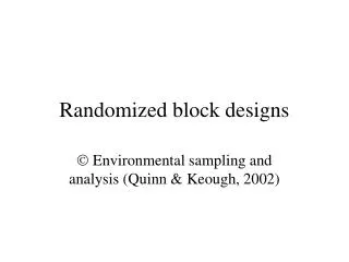
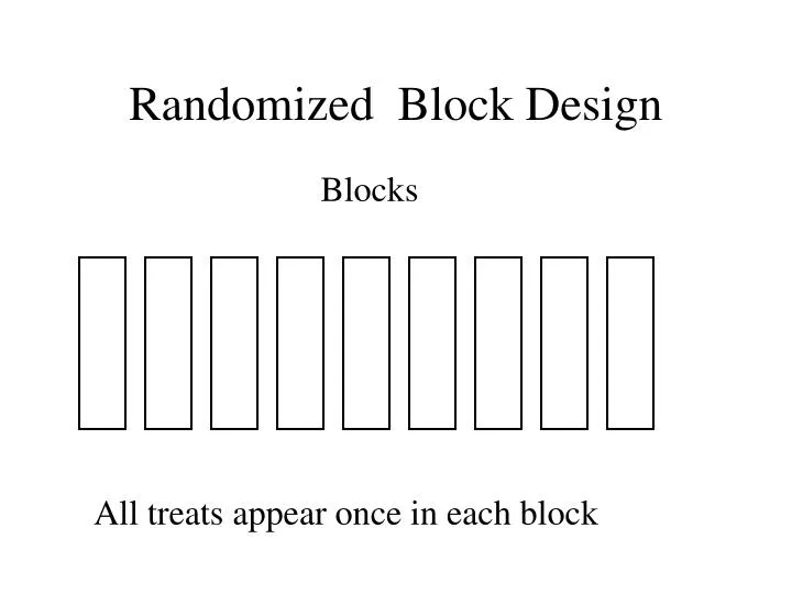
Randomized Block Design. Blocks. All treats appear once in each block. Latin Square Designs. Columns. Rows. The Latin square Design. All treats appear once in each row and each column. Latin Square Designs Selected Latin Squares 3 x 3 4 x 4 A B C A B C D A B C D A B C D A B C D

E N D
Randomized Block Design Blocks All treats appear once in each block
Columns Rows The Latin square Design All treats appear once in each row and each column
Latin Square Designs Selected Latin Squares 3 x 34 x 4 A B C A B C D A B C D A B C D A B C D B C A B A D C B C D A B D A C B A D C C A B C D B A C D A B C A D B C D A B D C A B D A B C D C B A D C B A 5 x 56 x 6 A B C D E A B C D E F B A E C D B F D C A E C D A E B C D E F B A D E B A C D A F E C B E C D B A F E B A D C
Definition • A Latin square is a square array of objects (letters A, B, C, …) such that each object appears once and only once in each row and each column. Example - 4 x 4 Latin Square. A B C D B C D A C D A B D A B C
In a Latin square You have three factors: • Treatments (t) (letters A, B, C, …) • Rows (t) • Columns (t) The number of treatments = the number of rows = the number of colums = t. The row-column treatments are represented by cells in a t x t array. The treatments are assigned to row-column combinations using a Latin-square arrangement
Example A courier company is interested in deciding between five brands (D,P,F,C and R) of car for its next purchase of fleet cars. • The brands are all comparable in purchase price. • The company wants to carry out a study that will enable them to compare the brands with respect to operating costs. • For this purpose they select five drivers (Rows). • In addition the study will be carried out over a five week period (Columns = weeks).
Each week a driver is assigned to a car using randomization and a Latin Square Design. • The average cost per mile is recorded at the end of each week and is tabulated below:
The Model for a Latin Experiment i = 1,2,…, t j = 1,2,…, t k = 1,2,…, t yij(k) = the observation in ith row and the jth column receiving the kth treatment m = overall mean tk = the effect of the ith treatment No interaction between rows, columns and treatments ri = the effect of the ith row gj = the effect of the jth column eij(k) = random error
A Latin Square experiment is assumed to be a three-factor experiment. • The factors are rows, columns and treatments. • It is assumed that there is no interaction between rows, columns and treatments. • The degrees of freedom for the interactions is used to estimate error.
Using SPSS for a Latin Square experiment Trts Rows Cols Y
Select the dependent variable and the three factors – Rows, Cols, Treats Select Model
Identify a model that has only main effects for Rows, Cols, Treats
Example2 In this Experiment thewe are again interested in how weight gain (Y) in rats is affected by Source of protein (Beef, Cereal, and Pork) and by Level of Protein (High or Low). There are a total of t = 3 X 2 = 6 treatment combinations of the two factors. • Beef -High Protein • Cereal-High Protein • Pork-High Protein • Beef -Low Protein • Cereal-Low Protein and • Pork-Low Protein
In this example we will consider using a Latin Square design Six Initial Weight categories are identified for the test animals in addition to Six Appetite categories. • A test animal is then selected from each of the 6 X 6 = 36 combinations of Initial Weight and Appetite categories. • A Latin square is then used to assign the 6 diets to the 36 test animals in the study.
A represents the high protein-cereal diet • B represents the high protein-pork diet • C represents the low protein-beef Diet • D represents the low protein-cereal diet • E represents the low protein-pork diet and • F represents the high protein-beef diet. In the latin square the letter
The weight gain after a fixed period is measured for each of the test animals and is tabulated below:
Diet SS partioned into main effects for Source and Level of Protein
Graeco-Latin Square Designs Mutually orthogonal Squares
Definition A Greaco-Latin square consists of two latin squares (one using the letters A, B, C, … the other using greek letters a, b, c, …) such that when the two latin square are supper imposed on each other the letters of one square appear once and only once with the letters of the other square. The two Latin squares are called mutually orthogonal. Example: a 7 x 7 Greaco-Latin Square Aa Be Cb Df Ec Fg Gd Bb Cf Dc Eg Fd Ga Ae Cc Dg Ed Fa Ge Ab Bf Dd Ea Fe Gb Af Bc Cg Ee Fb Gf Ac Bg Cd Da Ff Gc Ag Bd Ca De Eb Gg Ad Ba Ce Db Ef Fc
Note: At most (t –1) t x t Latin squares L1, L2, …, Lt-1 such that any pair are mutually orthogonal. It is possible that there exists a set of six 7 x 7 mutually orthogonal Latin squares L1, L2, L3, L4, L5, L6 .
The Greaco-Latin Square Design - An Example • the percentage of Lysine in the diet and • percentage of Protein in the diet • have on Milk Production in cows. A researcher is interested in determining the effect of two factors Previous similar experiments suggest that interaction between the two factors is negligible.
For this reason it is decided to use a Greaco-Latin square design to experimentally determine the two effects of the two factors (Lysine and Protein). • Seven levels of each factor is selected • 0.0(A), 0.1(B), 0.2(C), 0.3(D), 0.4(E), 0.5(F), and 0.6(G)% for Lysine and • 2(a), 4(b), 6(c), 8(d), 10(e), 12(f) and14(g)% for Protein ). • Seven animals (cows) are selected at random for the experiment which is to be carried out over seven three-month periods.
A Greaco-Latin Square is the used to assign the 7 X 7 combinations of levels of the two factors (Lysine and Protein) to a period and a cow. The data is tabulated on below:
The Model for a Greaco-Latin Experiment j = 1,2,…, t i = 1,2,…, t k = 1,2,…, t l = 1,2,…, t yij(kl) = the observation in ith row and the jth column receiving the kth Latin treatment and the lth Greek treatment
m = overall mean tk = the effect of the kth Latin treatment ll = the effect of the lth Greek treatment ri = the effect of the ith row gj = the effect of the jth column eij(k) = random error No interaction between rows, columns, Latin treatments and Greek treatments
A Greaco-Latin Square experiment is assumed to be a four-factor experiment. • The factors are rows, columns, Latin treatments and Greek treatments. • It is assumed that there is no interaction between rows, columns, Latin treatments and Greek treatments. • The degrees of freedom for the interactions is used to estimate error.
The Anova Table for a Greaco-Latin Square Experiment
Randomized Block Design • We want to compare t treatments • Group the N = bt experimentalunits into b homogeneous blocks of size t. • In each block we randomly assign the t treatments to the t experimental units in each block. • The ability to detect treatment to treatment differences is dependent on the within block variability.
Comments • The within block variability generally increases with block size. • The larger the block size the larger the within block variability. • For a larger number of treatments, t, it may not be appropriate or feasible to require the block size, k, to be equal to the number of treatments. • If the block size, k, is less than the number of treatments (k < t)then all treatments can not appear in each block. The design is called an Incomplete Block Design.
Commentsregarding Incomplete block designs • When two treatments appear together in the same block it is possible to estimate the difference in treatments effects. • The treatment difference is estimable. • If two treatments do not appear together in the same block it not be possible to estimate the difference in treatments effects. • The treatment difference may not be estimable.
Example • Consider the block design with 6 treatments and 6 blocks of size two. 1 2 2 3 1 3 4 5 5 6 4 6 • The treatments differences (1 vs 2, 1 vs 3, 2 vs 3, 4 vs 5, 4 vs 6, 5 vs 6) are estimable. • If one of the treatments is in the group {1,2,3} and the other treatment is in the group {4,5,6}, the treatment difference is not estimable.
Definitions • Two treatments i and i* are said to be connected if there is a sequence of treatments i0 = i, i1, i2, … iM = i* such that each successive pair of treatments (ij and ij+1) appear in the same block • In this case the treatment difference is estimable. • An incomplete design is said to be connected if all treatment pairs i and i* are connected. • In this case all treatment differences are estimable.
Example • Consider the block design with 5 treatments and 5 blocks of size two. 1 2 2 3 1 3 4 5 1 4 • This incomplete block design is connected. • All treatment differences are estimable. • Some treatment differences are estimated with a higher precision than others.
Definition An incomplete design is said to be a Balanced Incomplete Block Design. • if all treatments appear in exactly r blocks. • This ensures that each treatment is estimated with the same precision • The value of l is the same for each treatment pair. • if all treatment pairs i and i* appear together in exactly l blocks. • This ensures that each treatment difference is estimated with the same precision. • The value of l is the same for each treatment pair.
Some Identities Let b = the number of blocks. t = the number of treatments k = the block size r = the number of times a treatment appears in the experiment. l = the number of times a pair of treatment appears together in the same block • bk = rt • Both sides of this equation are found by counting the total number of experimental units in the experiment. • r(k-1) = l (t – 1) • Both sides of this equation are found by counting the total number of experimental units that appear with a specific treatment in the experiment.
BIB Design A Balanced Incomplete Block Design (b = 15, k = 4, t = 6, r = 10, l = 6)
An Example • For this purpose: • subjects will be asked to taste and compare these cereals scoring them on a scale of 0 - 100. • For practical reasons it is decided that each subject should be asked to taste and compare at most four of the six cereals. • For this reason it is decided to use b = 15 subjects and a balanced incomplete block design to assess the differences in taste of the six brands of cereal. A food processing company is interested in comparing the taste of six new brands (A, B, C, D, E and F) of cereal.
Analysis for the Incomplete Block Design Recall that the parameters of the design where b = 15, k = 4, t = 6, r = 10,l= 6 denotes summation over all blocks j containing treatment i.
Anova Table for Incomplete Block Designs Sums of Squares SS yij2 = 234382 S Bj2/k = 213188 S Qi2 = 181388.88 Anova Sums of Squares SStotal =SS yij2 –G2/bk = 27640.6 SSBlocks =S Bj2/k – G2/bk = 6446.6 SSTr = (S Qi2 )/(r – 1) = 20154.319 SSError = SStotal - SSBlocks - SSTr = 1039.6806
Designs for Estimating Carry-over (or Residual) Effects of Treatments