Download
1 / 21
210 likes | 502 Vues
"The impact of external market conditions on R&D valuation“ (by Lambert, Moreno and Platania) Discussed by Diego Ronchetti (University of Groningen). The literature has stressed (i) the importance of economic environment for R&D spending.

E N D
"The impact of external market conditions on R&D valuation“(by Lambert, Moreno and Platania)Discussed byDiego Ronchetti(University of Groningen)
The literature has stressed (i) the importance of economic environment for R&D spending • GDP as determinants of public spending in research and developments (Hammadou et al., 2014) • Public funding on innovative projects (Lanahan and Feldman, 2017) • Productivity growth and R&D expenses (e.g. Kancs an Siliverstovs, 2016)
and (ii) how and when to launch a project (entirely or in parts) • Staged investments (Majd and Pindyck, 1987) • Optimal timing of investment (McDonald and Siegel, 1986; Posner and Zuckerman, 1990) • Project’s market value (Berk et al. 2004) • Technical risk (Pindyck, 1993) • Cost of completion and expenditures (McDonald and Siegel, 1986; Pindyck, 1993) This paper proposes a project valuation method that accounts for changing economic environment
R&D project consisting of 2 phases R&D phase [0: tML) Idiosyncratic (technical, technological) risk (Tech risk) tML= Market launch date Market phase [tML:T] Systematic (economic) risk (Econ risk)
R&D phase [Tech risk] Poisson number of “test failures” K during development process If K > 0, null expected project value -> Tech risk premium Cash-flow discounting for failure risk
Market phase [Econ risk] f(t) = Fourier series Example: Φ = Econ risk-state vector (Φ = Φ[j] when f(t) has j terms) (discrete state vector) with PMF Examples in the paper: Business cycle indicators, VIX pj fixed to individual (or analysts’) expectation -> Econ risk premium Cash-flow discounting for econ risk
Market phase [Econ risk] f(t) = Fourier series representing econ risk Ct = net cash-flow stream after project approval {Wt} = Brownian motion as idiosyncratic risk-state variable process It = investment structure during R&D phase
Market phase [Econ risk] The project can be abandoned at each time during market phase: Abandon option value obtained by backward recursion: Both project value and embedded abandon option value depend on tML -> other things being equal, lower project value and higher option value if project launched just before a recession
Few points about the use of this valuation method for a R&D project
Econ risk: how do we determine its “true” nature? In the paper the “econ risk” for the net cash-flow stream after project approval derives from “external forces” Examples: Business Cycle [BC] indicators, VIX The selection of the “relevant external force” matters. Does the net cash-flow stream of the project follow more closely a financial cycle or a BC? They may differ
Econ risk: f(t) specification The duration of BCs varies. For example, in US: (data: National Bureau of Economic Research) Cyclical period of 5.35 years How long will the next cycle last? What about using "prediction sets“? July 1990 – March 2001
Other things being equal,the optimal project launch is just before a boom However, delaying project launch implies • Foregone patent protection • Risk of the introduction of a substitute good • Risk that a competitor conquers an important market share • Risk that the product is bypassed by a new product development -> Project value is affected by both market and competitors conditions What about discounting for these risks?
Diffusive process for the cash-flow What about extreme net cash-flow shocks? What about jumps?
"Can a Mimicking Synthetic Equity Structure Dominate the Risk Return Profile of Corporate Bonds?“(by Nouvellon and Pirotte)Discussed byDiego Ronchetti(University of Groningen)
This paper compares returns for - Corporate Bond Index (CBI)- Synthetic Equity Structure (SES) CBI • Weighted average of corporate bond prices • Constituents: bonds with a precise credit rating (AAA, AA, A, BBB, BB) • Investment: by entering a fund (aiming at) tracking the CBI • Contingent Claim Analysis: CBI as an option on the value A of the total assets of a representative firm with a precise credit rating -> Default occurs when A crosses a default barrier • Data: bond spreads from Merrill Lynch indexes -> Spreads implied probability of default (PD)
This paper compares returns for - Corporate Bond Index (CBI)- Synthetic Equity Structure (SES) SES replicating the CBI • Strategy to get CBI exposure without holding CBI itself • Constituents: equity index derivatives • Investment: by entering pooled fund structures holding the derivatives • SES as an option on an equity index with value S -> Structure stops occurs when S crosses a barrier • The index is the EURO STOXX 50 -> Model-implied PD
Results of the paper on- Corporate Bond Index (CBI)- Synthetic Equity Structure (SES) The authors find the for highly rated bonds we can have • Lower SES PD w.r.t. CBI • Higher SES yield w.r.t. CBI The authors conclude that for highly rated bonds (and corresponding low PD) SES has a better “spread/default” profile than CBI
Differences between CBI and SES • The SES barrier is not continuous (the index level is indeed observed just at few dates): the index level could go below and above the barrier level at intermediate times • Default barrier for CBI is continuous. The debt structure/repayment schedule for the chosen “bond index” may be continuous -> SES is safer as its PD is lower To keep the data: Why don’t consider the equity index values below the SES barrier as an “absorbing state” (looking back at each observation time)? To keep the SES: Why don’t take a single firm with (a) a precise repayment schedule matching the SES observation dates, and (b) without any credit need between two following observation dates?
Differences between CBI and SES • The CBI recovery amount is often paid years after default • The SES recovery amount is paid instantaneously -> SES pays more (that is, earlier) (Other things being equal) Why don’t discount the cash-flows by an "expected elapsed time" between default and recovery amount payment date?
Differences between CBI and SES • The SES’s underlying is an index build from equities of firms with distinct credit ratings • CBI is an index build from bonds with a chosen credit rating Isn’t “unfair” to compare SES with CBI from highly rated bonds? Why don’t create an index with equities of firms with a given credit rating?
Differences between CBI and SES What about the “average” liquidity for • a bond of a given credit rating (and then the CBI) • and that one of the assets necessary to implement the SES? -> No liquidity premium is now considered Why don’t include proxies for the liquidity of the assets when you discount the payoffs? Why don’t try to explain the “anomalous” spread/default SES profile by liquidity proxies?