Download
1 / 34
340 likes | 664 Vues
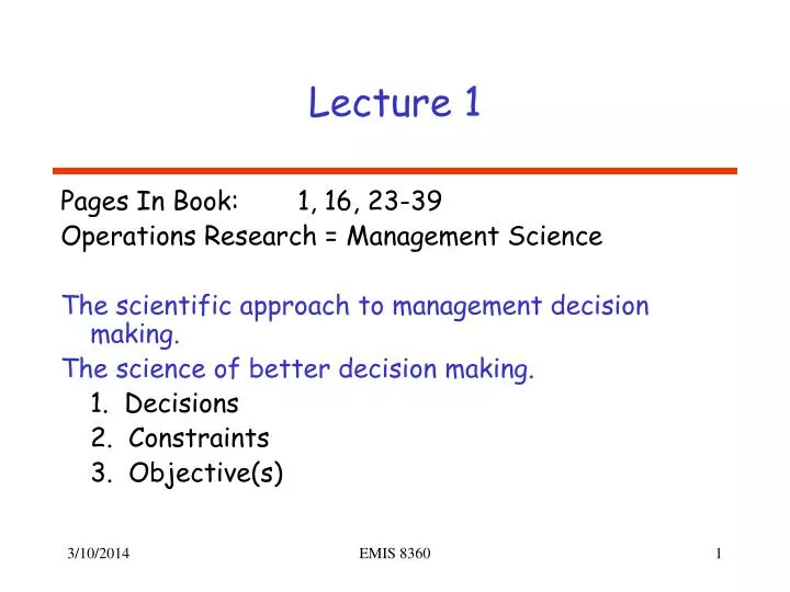
Lecture 1. Pages In Book: 1, 16, 23-39 Operations Research = Management Science The scientific approach to management decision making. The science of better decision making. 1. Decisions 2. Constraints 3. Objective(s). Section 1.6. Deterministic Models – all data are known

E N D
Lecture 1 Pages In Book: 1, 16, 23-39 Operations Research = Management Science The scientific approach to management decision making. The science of better decision making. 1. Decisions 2. Constraints 3. Objective(s) EMIS 8360
Section 1.6 Deterministic Models – all data are known Stochastic Models – quantities are known only by probability distributions Stochastic models are much more difficult to solve! (Example: point-to-point demand for service in a telecommunication data network) EMIS 8360
Chapter 2 Deterministic Optimization Models equal Mathematical Programs Composed Of The Following: 1. Subscripts 2. Constants and Sets 3. Decision Variables 4. Constraints 5. Objective Function EMIS 8360
Example 2.1 – Page 24 Subscripts (we only have one for this example) j – denotes the source of crude petroleum j = 1 implies Saudi Arabia j = 2 implies Venezuela EMIS 8360
Constants Conversion From Crude To Products EMIS 8360
Supply and Cost EMIS 8360
Demand – Must Be Met Each Day Units are barrels/day EMIS 8360
Decision Variables & Constraints X1 – denotes the number of barrels of Saudi crude processed each day X2 – denotes the number of barrels of Venezuela crude processed each day (Demand On Gasoline) 0.3X1 + 0.4X2> 2000 EMIS 8360
Constraints Continued (Demand On Jet Fuel) 0.4X1 + 0.2X2 > 1500 (Demand On Lubricants) 0.2X1 + 0.3X2> 500 (Max Supply From Saudi Arabia) X1< 9000 EMIS 8360
Constraints Continued (Max Supply From Venezuela) X2< 6000 (Non-negativity) X1> 0 X2 > 0 EMIS 8360
Objective Function (Minimize Cost) Minimize 20X1 + 15X2 Units = ($/barrel)(barrels) EMIS 8360
The Model Minimize 20X1 + 15X2 Subject To 0.3X1 + 0.4X2> 2000 0.4X1 + 0.2X2> 1500 0.2X1 + 0.3X2> 6000 0 < X1< 9000 0 < X2< 6000 EMIS 8360
The Graph X2 (000s) 0.3X1 + 0.4X2 = 2000 (6666.7,0) (0,5000) 0.3X1 + 0.4X2> 2000 8 6 4 2 X1 (000s) 2 4 6 8 EMIS 8360
The Graph - Continued X2 (000s) 0.4X1 + 0.2X2 = 1500 (3750,0) (0,7500) 0.4X1 + 0.2X2> 1500 8 6 4 2 X1 (000s) 2 4 6 8 EMIS 8360
The Graph - Continued X2 (000s) 0.2X1 + 0.3X2 = 500 (2500,0) (0,1666.7) 0.2X1 + 0.3X2> 500 Redundant! 8 6 4 2 X1 (000s) 2 4 6 8 EMIS 8360
The Graph - Continued X2 (000s) 0 < X1< 9000 0 < X2< 6000 Feasible Region 8 6 4 2 X1 (000s) 2 4 6 8 EMIS 8360
The Graph - Continued C = 20X1 + 15X2 X2 (000s) 8 6 4 2 X1 (000s) 2 4 6 8 EMIS 8360
The Graph - Continued X2 (000s) Optimum (2000, 3500) 8 6 0.3X1+0.4X2 = 2000 0.4X1+0.2X2 = 1500 Cost = 92,500 4 2 X1 (000s) 2 4 6 8 EMIS 8360
AMPL Software http://www.ampl.com Try AMPL download the Student Edition 2. (for Windows Users) amplcml.zip place this file in some directory – such as 8360/AMPL/ EMIS 8360
AMPL Software - Continued extract all to run double click sw Note: My model is in a:ex1.txt type sw: ampl ampl: model a:ex1.txt; EMIS 8360
Example in a:ex1.txt # AMPL Model Ex2.1 – a:ex1.txt option solver cplex; printf"AMPL Model Ex2.1 - run on PC\n\n"; var x1 >= 0, <= 9000; var x2 >= 0, <= 6000; minimize cost: 20*x1 + 15*x2; subject to Gas: 0.3*x1 + 0.4*x2 >= 2000; subject to Jet_Fuel: 0.4*x1 + 0.2*x2 >= 1500; subject to Lubricants: 0.2*x1 + 0.3*x2 >= 500; expand cost; expand Gas; expand Jet_Fuel; expand Lubricants; solve; display x1; display x2; EMIS 8360
Solution Obtained ampl: model a:ex1.txt; AMPL Model Ex2.1 - run on PC minimize cost: 20*x1 + 15*x2; subject to Gas: 0.3*x1 + 0.4*x2 >= 2000; subject to Jet_Fuel: 0.4*x1 + 0.2*x2 >= 1500; subject to Lubricants: 0.2*x1 + 0.3*x2 >= 500; CPLEX 8.0.0: optimal solution; objective 92500 2 dual simplex iterations (0 in phase I) x1 = 2000 x2 = 3500 EMIS 8360
To Save Solution While still in sw: use edit to select all use edit to copy then paste to Word or notepad document then you can turn in your output EMIS 8360
Generic Model The generic model does not have the data with the model. The data is in a separate file. Hence we can solve any problem of this type. We simply provide the proper data in a data file. EMIS 8360
# Ex2.1 AMPL Model - Generic - a:ex2.txt option solver cplex; set S; # sourses - sa = Saudi Arabia, v = Venezuela set P; # products - g = gas, j = jet fuel, l = lubs param a {S}; # availability of crude from sources param c {S}; # cost/barrel param d {P}; # demand for products param cf {S,P}; # conversion factor - crude to product data a:data.txt; var x {s in S} >= 0, <= a[s]; minimize cost: sum {s in S} c[s]*x[s]; subject to Demand {p in P}: sum {s in S} cf[s,p]*x[s] >= d[p]; solve; display x; expand cost; expand Demand; EMIS 8360
# Ex2.1 AMPL Model - Generic - a:data.txt set S := sa v; set P := g j l; param a := sa 9000 v 6000; param c := sa 20 v 15; param d := g 2000 j 1500 l 500; param cf := sa g 0.3 v g 0.4 sa j 0.4 v j 0.2 sa l 0.2 v l 0.3; EMIS 8360
ampl: model a:ex2.txt; CPLEX 8.0.0: optimal solution; objective 92500 2 dual simplex iterations (0 in phase I) x [*] := sa 2000 v 3500; minimize cost: 20*x['sa'] + 15*x['v']; subject to Demand['g']: 0.3*x['sa'] + 0.4*x['v'] >= 2000; subject to Demand['j']: 0.4*x['sa'] + 0.2*x['v'] >= 1500; subject to Demand['l']: 0.2*x['sa'] + 0.3*x['v'] >= 500; EMIS 8360
Optimal Solutions For Linear Programs (LPs) There will be either a unique optimum or an infinite number of optimal solutions. There cannot be exactly 2 optimal solutions to a LP. EMIS 8360
Unique Solution Max 2X + Y Subject To X + Y < 5 0 < X < 3 0 < Y < 4 optimum EMIS 8360
Infinite Number Of Solutions All points are optimal Max 2X + 2Y Subject To X + Y < 5 0 < X < 3 0 < Y < 4 EMIS 8360
Output From AMPL For An Infinite Number Of Solutions # Example With An Infinite Number Of Solutions # runL1c.txt option solver cplex; var X >= 0, <= 3; var Y >= 0, <= 4; maximize profit: 2*X + 2*Y; subject to Constraint: X + Y <= 5; expand profit; expand Constraint; solve; display X, Y; EMIS 8360
Output Is A Single Solution sw: ampl ampl: model runL1c.txt; maximize profit: 2*X + 2*Y; s.t. Constraint: X + Y <= 5; CPLEX 7.1.0: optimal solution; objective 10 0 simplex iterations (0 in phase I) X = 3 Y = 2 ampl: Other Optimal Solutions: (1,4), (2,3),(1.5,3.5), Etc. EMIS 8360
Example Of A Problem With No Feasible Solutions max X subject To: X + Y < 2 X + Y > 4 X > 0, Y > 0 EMIS 8360
Example Of An Unbounded Problem Max X Subject To: X + Y > 10 X > 0 0 < Y < 10 Try (100,5), (1000, 7) (10000, 10) EMIS 8360