Download
1 / 53
560 likes | 1.12k Vues
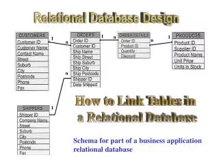
Relational Database Design. Functional Dependencies and Normalization. Relational Database Design. Pitfalls in Relational Database Design Functional Dependencies Decomposition Normal Forms Designing a Set of Relations. Pitfalls in Relational Database Design.

E N D
Relational Database Design Functional Dependencies and Normalization
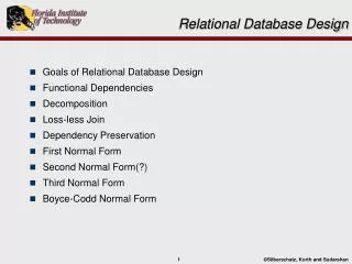
Relational Database Design • Pitfalls in Relational Database Design • Functional Dependencies • Decomposition • Normal Forms • Designing a Set of Relations
Pitfalls in Relational Database Design • Relational database design requires that we find a “good” collection of relation schemas. A bad design may lead to • Repetition of Information. • Inability to represent certain information. • Design Goals: • Avoid redundant data • Ensure that relationships among attributes are represented • Facilitate the checking of updates for violation of database integrity constraints.
Example • Consider the relation schema: • Redundancy: • Data for DNUMER, DNAME, DMGRSSN are repeated for each employee who works for that department. • Wastes space • Update anomalies
Example of an Update Anomaly • Consider the relation: • Insertion Anomaly: • Cannot insert a new department that has no employees as yet. • Using NULL values causes other difficulties • Deletion Anomaly: if we delete the last employee who works for a department, the information concerning that department is lost. • Update Anomaly: Updating the value of one of the attributes of a department requires updating the tuples of all employees who work in that department.
Decomposition • Decompose the relation schemainto: • All attributes of an original schema (R) must appear in the decomposition (R1, R2): R = R1 R2 • Lossless-join decomposition.For all possible relations r on schema R r = R1 (r) R2 (r)
Example of Non Lossless-Join Decomposition • Decomposition of R = (A, B) R1 = (A) R2 = (B) A B A B 1 2 1 1 2 B(r) A(r) r A B A (r) B (r) 1 2 1 2
Goal • Decide whether a particular relation R is in “good” form. • In the case that a relation R is not in “good” form, decompose it into a set of relations {R1, R2, ..., Rn} such that • each relation is in good form • the decomposition is a lossless-join decomposition • Our theory is based on: • functional dependencies • multivalued dependencies
Functional Dependencies • Constraints on the set of legal relations. • Require that the value for a certain set of attributes determines uniquely the value for another set of attributes. • A functional dependency is a generalization of the notion of a key.
Functional Dependencies (Cont.) • Let R be a relation schema R and R • The functional dependency holds onR if and only if for any legal relations r(R), whenever any two tuples t1and t2 of r agree on the attributes , they also agree on the attributes . That is, t1[] = t2 [] t1[ ] = t2 [ ] • Example: Consider r(A,B) with the following instance of r. • On this instance, AB does NOT hold, but BA does hold. • 4 • 1 5 • 3 7
Functional Dependencies (Cont.) • K is a superkey for relation schema R if and only if K R • K is a candidate key for R if and only if • K R, and • for no K, R • Functional dependencies allow us to express constraints that cannot be expressed using superkeys. Consider the schema: We expect this set of functional dependencies to hold: SSNENAME DNUMBER {DNAME, DMGRSSN}
Use of Functional Dependencies • We use functional dependencies to: • test relations to see if they are legal under a given set of functional dependencies. • If a relation r is legal under a set F of functional dependencies, we say that rsatisfies F. • specify constraints on the set of legal relations • We say that Fholds onR if all legal relations on R satisfy the set of functional dependencies F. • Note: A specific instance of a relation schema may satisfy a functional dependency even if the functional dependency does not hold on all legal instances. For example, a specific instance of EMP_DEPT may, by chance, satisfy ENAME BDATE.
Functional Dependencies (Cont.) • A functional dependency is trivial if it is satisfied by all instances of a relation • E.g. • ENAME, BDATE ENAME • ADDRESS ADDRESS • In general, is trivial if
Closure of a Set of Functional Dependencies • Given a set F set of functional dependencies, there are certain other functional dependencies that are logically implied by F. • E.g. If A B and B C, then we can infer that A C • The set of all functional dependencies logically implied by F is the closure of F. We denote the closure of F by F+. • We can find all ofF+by applying Armstrong’s Axioms: • if , then (reflexivity) • if , then (augmentation) • if , and , then (transitivity) • These rules are • sound (generate only functional dependencies that actually hold) and • complete (generate all functional dependencies that hold).
Example • R = (A, B, C, G, H, I)F = { A BA CCG HCG IB H} • some members of F+ • A H • by transitivity from A B and B H • AG I • by augmenting A C with G, to get AG CG and then transitivity with CG I • CG HI • from CG H and CG I : “union rule” can be inferred from • definition of functional dependencies, or • Augmentation of CG I to infer CG CGI, augmentation ofCG H to inferCGI HI, and then transitivity
To compute the closure of a set of functional dependencies F: F+ = Frepeatfor each functional dependency f in F+ apply reflexivity and augmentation rules on fadd the resulting functional dependencies to F+for each pair of functional dependencies f1and f2 in F+iff1 and f2 can be combined using transitivitythen add the resulting functional dependency to F+until F+ does not change any further NOTE: We will see an alternative procedure for this task later Procedure for Computing F+
Closure of Functional Dependencies (Cont.) • We can further simplify manual computation of F+ by using the following additional rules. • If holdsand holds, then holds (union) • If holds, then holds and holds (decomposition) • If holdsand holds, then holds (pseudotransitivity) The above rules can be inferred from Armstrong’s axioms.
Closure of Attribute Sets • Given a set of attributes a, define the closureof aunderF (denoted by a+) as the set of attributes that are functionally determined by a under F: ais in F+ a+ • Algorithm to compute a+, the closure of a under F result := a;while (changes to result) do for each in F do begin if result then result := result end
Example of Attribute Set Closure • R = (A, B, C, G, H, I) • F = {A BA CCG HCG IB H} • (AG)+ 1. result = AG 2. result = ABCG (A C and A B) 3. result = ABCGH (CG H and CG AGBC) 4. result = ABCGHI (CG I and CG AGBCH) • Is AG a candidate key? • Is AG a super key? • Does AG R? • Is any subset of AG a superkey? • Does A+R? • Does G+R?
There are several uses of the attribute closure algorithm: Testing for superkey: To test if is a superkey, we compute +, and check if + contains all attributes of R. Testing functional dependencies To check if a functional dependency holds (or, in other words, is in F+), just check if +. That is, we compute + by using attribute closure, and then check if it contains . Is a simple and cheap test, and very useful Computing closure of F For each R, we find the closure +, and for each S +, we output a functional dependency S. Uses of Attribute Closure
Canonical Cover • Sets of functional dependencies may have redundant dependencies that can be inferred from the others • Eg: A C is redundant in: {A B, B C, A C} • Parts of a functional dependency may be redundant • E.g. on RHS: {A B, B C, A CD} can be simplified to {A B, B C, A D} • E.g. on LHS: {A B, B C, AC D} can be simplified to {A B, B C, A D} • Intuitively, a canonical cover of F is a “minimal” set of functional dependencies equivalent to F, with no redundant dependencies or having redundant parts of dependencies
Extraneous Attributes • Consider a set F of functional dependencies and the functional dependency in F. • Attribute A is extraneous in if A and F logically implies (F – {}) {( – A) }. • Attribute A is extraneous in if A and the set of functional dependencies (F – {}) {(– A)} logically implies F. • Note: implication in the opposite direction is trivial in each of the cases above, since a “stronger” functional dependency always implies a weaker one. • Example: Given F = {AC, ABC } • B is extraneous in AB C because AC logically impliesABC. • Example: Given F = {AC, ABCD} • C is extraneous in ABCD since AC can be inferred even after deleting C.
Testing if an Attribute is Extraneous • Consider a set F of functional dependencies and the functional dependency in F. • To test if attribute A is extraneousin • compute ( – {A})+ using the dependencies in F • check that ( – {A})+ contains ; if it does, A is extraneous • To test if attribute A is extraneous in • compute + using only the dependencies in F’ = (F – {}) {(– A)}, • check that + contains A; if it does, A is extraneous
Canonical Cover • A canonical coverfor F is a set of dependencies Fc such that • F logically implies all dependencies in Fc, and • Fclogically implies all dependencies in F, and • No functional dependency in Fccontains an extraneous attribute, and • Each left side of functional dependency in Fcis unique. • To compute a canonical cover for F: 1. Replace each functional dependency {A1, A2,…, An} in F by the n functional dependencies A1, A2,…, An 2. For each functional dependency A in F For each B , if {{F{ A}}{({B}) A}} is equivalent to F, then replace A with ({B}) A} in F. 3. For each remaining functional dependency A in F If {F{ A}} is equivalent to F, then remove A from F.
Example of Computing a Canonical Cover • R = (A, B, C)F = {A BC B C A BABC} • Replace A BC with A B and A C • Set is now {A B, A C, B C, ABC} • A is extraneous in ABC because BC logically implies AB C. • Set is now {A B, A C, B C} • A C is redundant since it is logically implied by A B and B C. • The canonical cover is: A B B C
Decomposition • All attributes of an original schema (R) must appear in the decomposition (R1, R2): R = R1 R2 • Lossless-join decomposition.For all possible relations r on schema R r = R1 (r) R2 (r) • A decomposition of R into R1 and R2 is lossless join if and only if at least one of the following dependencies is in F+: • R1 R2R1 • R1 R2R2
A B A B 1 2 1 1 2 B(r) A(r) r A B A (r) B (r) 1 2 1 2 Example of Lossy-Join Decomposition • Lossy-join decompositions result in information loss. • Example: Decomposition of R = (A, B) R2 = (A) R2 = (B)
Introduction to Normalization • Normalization: Process of decomposing unsatisfactory "bad" relations by breaking up their attributes into smaller relations • Normal form: Condition using keys and FDs of a relation to certify whether a relation schema is in a particular normal form • 2NF, 3NF, BCNF based on keys and FDs of a relation schema • 4NF based on keys, multi-valued dependencies: MVDs; 5NF based on keys, join dependencies : JDs • Additional properties may be needed to ensure a good relational design (lossless join, dependency preservation)
Normalization Using Functional Dependencies • When we decompose a relation schema R with a set of functional dependencies F into R1, R2,.., Rn we want • Lossless-join decomposition: Otherwise decomposition would result in information loss. • No redundancy: The relations Ripreferably should be in either Boyce-Codd Normal Form or Third Normal Form. • Dependency preservation: Let Fibe the set of dependencies F+ that include only attributes in Ri. • Preferably the decomposition should be dependency preserving, that is, (F1 F2 … Fn)+ = F+ • Otherwise, checking updates for violation of functional dependencies may require computing joins, which is expensive.
First Normal Form • A relational schema R is in first normal form if the domains of all attributes of R are atomic: Disallow composite attributes, multivalued attributes, and nested relations; attributes whose values for an individual tuple are non-atomic • Considered to be part of the definition of relation
Second Normal Form • Uses the concepts of FDs, primary key Definitions: • Prime attribute - attribute that is member of the primary key K • Full functional dependency - a FD Y Z where removal of any attribute from Y means the FD does not hold any more Examples: - {SSN, PNUMBER} HOURS is a full FD since neither SSN HOURS nor PNUMBER HOURS hold - {SSN, PNUMBER} ENAME is not a full FD (it is called a partial dependency) since SSN ENAME also holds • A relation schema R is in second normal form (2NF) if every non-prime attribute A in R is fully functionally dependent on the primary key.
Third Normal Form • Transitive functional dependency - a FD X Z that can be derived from two FDs X Y and Y Z Examples: SSN DMGRSSN is a transitive FD since SSN DNUMBER and DNUMBER DMGRSSN hold SSN ENAME is non-transitive since there is no set of attributes X where SSN X and X ENAME • A relation schema R is in third normal form (3NF) if it is in 2NF and no non-prime attribute A in R is transitively dependent on the primary key. NOTE: • InX Y and Y Z, with X as the primary key, we consider this a problem only if Y is not a candidate key. When Y is a candidate key, there is no problem with the transitive dependency . E.g., Consider EMP (SSN, Emp#, Salary). Here, SSN Emp# Salary and Emp# is a candidate key.
Decomposition Example • R = (A, B, C)F = {A B, B C) • R1 = (A, B), R2 = (B, C) • Lossless-join decomposition: R1 R2 = {B} and B BC • Dependency preserving • R1 = (A, B), R2 = (A, C) • Lossless-join decomposition: R1 R2 = {A} and A AB • Not dependency preserving (cannot check B C without computing R1 R2)
To check if a dependency is preserved in a decomposition of R into R1, R2, …, Rn we apply the following simplified test (with attribute closure done w.r.t. F) result = while (changes to result) dofor eachRiin the decompositiont = (result Ri)+ Riresult = result t If result contains all attributes in , then the functional dependency is preserved. We apply the test on all dependencies in F to check if a decomposition is dependency preserving This procedure takes polynomial time, instead of the exponential time required to compute F+and(F1 F2 … Fn)+ Testing for Dependency Preservation
Boyce-Codd Normal Form • is trivial (i.e., ) • is a superkey for R A relation schema R is in BCNF with respect to a set F of functional dependencies if for all functional dependencies in F+ of the form , where R and R,at least one of the following holds:
Example • R = (A, B, C)F = {AB B C}Key = {A} • R is not in BCNF • Decomposition R1 = (A, B), R2 = (B, C) • R1and R2 in BCNF • Lossless-join decomposition • Dependency preserving
Testing for BCNF • To check if a non-trivial dependency causes a violation of BCNF 1. compute + (the attribute closure of ), and 2. verify that it includes all attributes of R, that is, it is a superkey of R.
BCNF Decomposition Algorithm result := {R};done := false;compute F+;while (not done) do if (there is a schema Riin result that is not in BCNF)then beginlet be a nontrivial functional dependency that holds on Risuch that Riis not in F+, and = ;result := (result – Ri) (Ri – ) (, );end else done := true; Note: each Riis in BCNF, and decomposition is lossless-join.
Example of BCNF Decomposition • R = (A, B, C, D, E, F)F = {A C B E F A}Key = {D, E} • Decomposition • R1 = (A, B, C) • R2 = (A, D, E, F) • R3 = (A, E, F) • R4 = (D, E) • Final decomposition R1, R3, R4
Testing Decomposition for BCNF • To check if a relation Ri in a decomposition of R is in BCNF, • Either test Ri for BCNF with respect to the restriction of F to Ri (that is, all FDs in F+ that contain only attributes from Ri) • or use the original set of dependencies F that hold on R, but with the following test: • for every set of attributes Ri, check that + (the attribute closure of ) either includes no attribute of Ri- , or includes all attributes of Ri. • If the condition is violated by some in F, the dependency (+ - ) Rican be shown to hold on Ri, and Ri violates BCNF. • We use above dependency to decompose Ri
BCNF and Dependency Preservation It is not always possible to get a BCNF decomposition that is dependency preserving • R = (J, K, L)F = {JK L L K}Two candidate keys = JK and JL • R is not in BCNF • Any decomposition of R will fail to preserve JK L
Third Normal Form: Motivation • There are some situations where • BCNF is not dependency preserving, and • efficient checking for FD violation on updates is important • Solution: define a weaker normal form, called Third Normal Form. • Allows some redundancy (with resultant problems; we will see examples later) • But FDs can be checked on individual relations without computing a join. • There is always a lossless-join, dependency-preserving decomposition into 3NF.
Third Normal Form • A relation schema R is in third normal form (3NF) if for all: in F+at least one of the following holds: • is trivial (i.e., ) • is a superkey for R • Each attribute A in – is contained in a candidate key for R. (NOTE: each attribute may be in a different candidate key) • If a relation is in BCNF it is in 3NF (since in BCNF one of the first two conditions above must hold). • Third condition is a minimal relaxation of BCNF to ensure dependency preservation (will see why later).
3NF (Cont.) • Example • R = (J, K, L)F = {JK L, L K} • Two candidate keys: JK and JL • R is in 3NF JK L JK is a superkeyL K K is contained in a candidate key • BCNF decomposition has (JL) and (LK) • Testing for JK L requires a join • There is some redundancy in this schema.
Testing for 3NF • Optimization: Need to check only FDs in F, need not check all FDs in F+. • Use attribute closure to check, for each dependency , if is a superkey. • If is not a superkey, we have to verify if each attribute in is contained in a candidate key of R • this test is rather more expensive, since it involve finding candidate keys • testing for 3NF has been shown to be NP-hard • Interestingly, decomposition into third normal form (described shortly) can be done in polynomial time
3NF Decomposition Algorithm Let Fcbe a canonical cover for F;i := 0;for each functional dependency in Fcdo if none of the schemas Rj, 1 j i contains then begini := i + 1;Ri := endif none of the schemas Rj, 1 j i contains a candidate key for Rthen begini := i + 1;Ri := any candidate key for R;end return (R1, R2, ..., Ri)
3NF Decomposition Algorithm (Cont.) • Above algorithm ensures: • each relation schema Riis in 3NF • decomposition is dependency preserving and lossless-join
Example • Relation schema: R = (A, B, C, D) • The functional dependencies for this relation schema are:C A D B A C • The key is: {B, A} • The for loop in the algorithm causes us to include the following schemas in our decomposition: T = (C, A,D) S = (B, A, C) • Since S contains a candidate key for R, we are done with the decomposition process.
Comparison of BCNF and 3NF • It is always possible to decompose a relation into relations in 3NF and • the decomposition is lossless • the dependencies are preserved • It is always possible to decompose a relation into relations in BCNF and • the decomposition is lossless • it may not be possible to preserve dependencies.
J L K j1 j2 j3 null l1 l1 l1 l2 k1 k1 k1 k2 Comparison of BCNF and 3NF (Cont.) • Example of problems due to redundancy in 3NF • R = (J, K, L)F = {JK L, L K} A schema that is in 3NF but not in BCNF has the problems of • repetition of information (e.g., the relationship l1, k1) • need to use null values (e.g., to represent the relationshipl2, k2 where there is no corresponding value for J).