Download
1 / 41
490 likes | 1.26k Vues
Semi-Classical Transport Theory. Outline:. What is Computational Electronics? Semi-Classical Transport Theory Drift-Diffusion Simulations Hydrodynamic Simulations Particle-Based Device Simulations Inclusion of Tunneling and Size-Quantization Effects in Semi-Classical Simulators

E N D
Outline: • What is Computational Electronics? • Semi-Classical Transport Theory • Drift-Diffusion Simulations • Hydrodynamic Simulations • Particle-Based Device Simulations • Inclusion of Tunneling and Size-Quantization Effects in Semi-Classical Simulators • Tunneling Effect: WKB Approximation and Transfer Matrix Approach • Quantum-Mechanical Size Quantization Effect • Drift-Diffusion and Hydrodynamics: Quantum Correction and Quantum Moment Methods • Particle-Based Device Simulations: Effective Potential Approach • Quantum Transport • Direct Solution of the Schrodinger Equation (Usuki Method) and Theoretical Basis of the Green’s Functions Approach (NEGF) • NEGF: Recursive Green’s Function Technique and CBR Approach • Atomistic Simulations – The Future • Prologue
Semi-Classical Transport Theory • It is based on direct or approximate solution of the Boltzmann Transport Equation for the semi-classical distribution function f(r,k,t) which gives one the probability of finding a particle in region (r,r+dr) and (k,k+dk) at time t • Moments of the distribution function give us information about: • Particle Density • Current Density • Energy Density D. K. Ferry, Semiconductors, MacMillian, 1990.
Semi-Classical Transport Approaches 1. Drift-Diffusion Method 2. Hydrodynamic Method 3. Direct Solution of the Boltzmann Transport Equation via: • Particle-Based Approaches – Monte Carlo method • Spherical Harmonics • Numerical Solution of the Boltzmann-Poisson Problem C. Jacoboni, P. Lugli: "The Monte Carlo Method for Semiconductor Device Simulation“, in series "Computational Microelectronics", series editor: S. Selberherr; Springer, 1989, ISBN: 3-211-82110-4.
1. Drift-Diffusion Approach Constitutive Equations • Poisson • Continuity Equations • Current Density Equations S. Selberherr: "Analysis and Simulation of Semiconductor Devices“, Springer, 1984.
Numerical Solution Details • Linearization of the Poisson equation • Scharfetter-Gummel Discretization of the Continuity equation • De Mari scaling of variables • Discretization of the equations • Finite Difference – easier to implement but requires more node points, difficult to deal with curved interfaces • Finite Elements – standard, smaller number of node points, resolves curved surfaces • Finite Volume
Linearized Poisson Equation φ→φ + δ where δ= φnew - φold • Finite difference discretization: • Potential varies linearly between mesh points • Electric field is constant between mesh points • Linearization → Diagonally-dominant coefficient matrix A is obtained
Scharfetter-Gummel Discretization of the Continuity Equation • Electron and hole densities n and p vary exponentially between mesh points → relaxes the requirement of using very small mesh sizes • The exponential dependence of n and p upon the potential is buried in the Bernoulli functions Bernoulli function:
Numerical Solution Details Governing Equations ICS/BCS System of Algebraic Equations Equation (Matrix) Solver ApproximateSolution Discretization φi (x,y,z,t) p (x,y,z,t) n (x,y,z,t) Continuous Solutions Finite-Difference Finite-Volume Finite-Element Spectral Boundary Element Hybrid Discrete Nodal Values Tridiagonal SOR Gauss-Seidel Krylov Multigrid D. Vasileska, EEE533 Semiconductor Device and Process Simulation Lecture Notes, Arizona State University, Tempe, AZ.
Numerical Solution Details • Poisson solvers: • Direct • Gaussian Eliminatioln • LU decomposition • Iterative • Mesh Relaxation Methods • Jacobi, Gauss-Seidel, Successive over-Relaxation • Advanced Iterative Solvers • ILU, Stone’s strongly implicit method, Conjugate gradient methods and Multigrid methods G. Speyer, D. Vasileska and S. M. Goodnick, "Efficient Poisson solver for semiconductor device modeling using the multi-grid preconditioned BICGSTAB method", Journal of Computational Electronics, Vol. 1, pp. 359-363 (2002).
n1/2 n1/3 Complexity of linear solvers Time to solve model problem (Poisson’s equation) on regular mesh
Numerical Solution Details of the Coupled Equation Set • Solution Procedures: • Gummel’s Approach – when the constitutive equations are weekly coupled • Newton’s Method – when the constitutive equations are strongly coupled • Gummel/Newton – more efficient approach D. Vasileska and S. M. Goodnick,Computational Electronics, Morgan & Claypool, 2006. D. Vasileska, S. M. Goodnick and G. Klimeck, Computational Electronics: From Semiclassical to Quantum Transport Modeling, Taylor & Francis, in press.
Constraints on the MESH Size and TIME Step The time step and the mesh size may correlate to each other in connection with the numerical stability: • The time step t must be related to the plasma frequency • The Mesh size is related to the Debye length
When is the Drift-Diffusion Model Valid? • Large devices where the velocity of the carriers is smaller than the saturation velocity • The validity of the method can be extended for velocity saturated devices as well by introduction of electric field dependent mobility and diffusion coefficient: Dn(E) and μn(E) 100 nm 25 nm 140 nm
What Contributes to The Mobility? D. Vasileska and S. M. Goodnick, "Computational Electronics", Materials Science and Engineering, Reports: A Review Journal, Vol. R38, No. 5, pp. 181-236 (2002)
Mobility Modeling Mobility modeling can be separated in three parts: • Low-field mobility characterization for bulk or inversion layers • High-field mobility characterization to account for velocity saturation effect • Smooth interpolation between the low-field and high-field regions Silvaco ATLAS Manual.
(A) Low-Field Models for Bulk Materials Phonon scattering: - Simple power-law dependence of the temperature - Sah et al. model: acoustic + optical and intervalley phonons combined via Mathiessen’s rule Ionized impurity scattering: - Conwell-Weiskopf model - Brooks-Herring model
(A) Low-Field Models for Bulk Materials (cont’d) Combined phonon and ionized impurity scattering: - Dorkel and Leturg model: temperature-dependent phonon scattering +ionized impurity scattering + carrier-carrier interactions - Caughey and Thomas model: temperature independent phonon scattering + ionized impurity scattering
(A) Low-Field Models for Bulk Materials (cont’d) - Sharfetter-Gummel model: phonon scattering + ionized impurity scattering (parameterized expression – does not use the Mathiessen’s rule) - Arora model: similar to Caughey and Thomas, but with temperature dependent phonon scattering
(A) Low-Field Models for Bulk Materials (cont’d) Carrier-carrier scattering - modified Dorkel and Leturg model Neutral impurity scattering: - Li and Thurber model: mobility component due to neutral impurity scattering is combined with the mobility due to lattice, ionized impurity and carrier-carrier scattering via the Mathiessen’s rule
(C) Inversion Layer Mobility Models • CVT model: • combines acoustic phonon, non-polar optical phonon and surface-roughness scattering (as an inverse square dependence of the perpendicular electric field) via Mathiessen’s rule • Yamaguchi model: • low-field part combines lattice, ionized impurity and surface-roughness scattering • there is also a parametric dependence on the in-plane field (high-field component)
(C) Inversion Layer Mobility Models (cont’d) • Shirahata model: • uses Klaassen’s low-field mobility model • takes into account screening effects into the inversion layer • has improved perpendicular field dependence for thin gate oxides • Tasch model: • the best model for modeling the mobility in MOS inversion layers; uses universal mobility behavior
Hydrodynamic Modeling • In small devices there exists non-stationary transport and carriers are moving through the device with velocity larger than the saturation velocity • In Si devices non-stationary transport occurs because of the different order of magnitude of the carrier momentum and energy relaxation times • In GaAs devices velocity overshoot occurs due to intervalley transfer T. Grasser (ed.): "Advanced Device Modeling and Simulation“, World Scientific Publishing Co., 2003, ISBN: 9-812-38607-6 M. M. Lundstrom, Fundamentals of Carrier Transport, 1990.
Velocity Overshoot in Silicon • Scattering mechanisms: • Acoustic deformation potential scattering • Zero-order intervalley scattering (f and g-phonons) • First-order intervalley scattering (f and g-phonons) X. He, MS Thesis, ASU, 2000.
How is the Velocity Overshoot Accounted For? • In Hydrodynamic/Energy balance modeling the velocity overshoot effect is accounted for through the addition of an energy conservation equation in addition to: • Particle Conservation (Continuity Equation) • Momentum (mass) Conservation Equation
Hydrodynamic Model due to Blotakjer Constitutive Equations: Poisson +
Momentum Relaxation Rate K. Tomizawa, Numerical Simulation Of Submicron Semiconductor Devices.
Energy Relaxation Rate K. Tomizawa, Numerical Simulation Of Submicron Semiconductor Devices.
Validity of the Hydrodynamic Model 90 nm device SR = series resistance Silvaco ATLAS simulations performed by Prof. Vasileska.
Validity of the Hydrodynamic Model 25 nm device SR = series resistance Silvaco ATLAS simulations performed by Prof. Vasileska.
Validity of the Hydrodynamic Model 14 nm device SR = series resistance Silvaco ATLAS simulations performed by Prof. Vasileska.
Failure of the Hydrodynamic Model 14 nm 25 nm 90 nm Silvaco ATLAS simulations performed by Prof. Vasileska.
Failure of the Hydrodynamic Model 14 nm 25 nm 90 nm Silvaco ATLAS simulations performed by Prof. Vasileska.
Failure of the Hydrodynamic Model 14 nm 25 nm 90 nm Silvaco ATLAS simulations performed by Prof. Vasileska.
Summary • Drift-Diffusion model is good for large MOSFET devices, BJTs, Solar Cells and/or high frequency/high power devices that operate in the velocity saturation regime • Hydrodynamic model must be used with caution when modeling devices in which velocity overshoot, which is a signature of non-stationary transport, exists in the device • Proper choice of the energy relaxation times is a problem in hydrodynamic modeling