Download
1 / 24
240 likes | 407 Vues
2. The work reported here was developed under the STAR Research Assistance Agreement CR-829095 awarded by the U.S. Environmental Protection Agency (EPA) to Colorado State University. This presentation has not been formally reviewed by EPA.

E N D
1. 1
2. 2 Project Funding
3. 3 Context: Section 303(d) CWA Assessment of water quality.
Identify water bodies for which controls are not stringent enough for the health of indigenous shellfish, fish and wildlife.
TMDL assessments ��a margin of safety which takes into account any lack of knowledge��
4. 4 Specific Points Meetings and Collaborations
Computational Issues in Bayes Networks
Spatial Correlation in Bayes Networks
5. 5 Meetings and Collaborations Ken Reckhow; Director, Water Resources Research Institute of the University of North Carolina & Professor, Water Resources at Duke University
Implemented Bayes Network models for the Neuse River Watershed
Evaluate TMDL standards, Suggest future monitoring
July/August 2003 issue of the Journal of Water Resources Planning and Management
6. 6 Meetings and Collaborations JoAnn Hanowski, Natural Resources Research Institute, University of Minnesota at Duluth
Avian ecology (Great Lakes)
Point count data
Data at landscape and smaller scales
7. 7 Computational Issues Check out Steve Jensen�s poster on computational issues for Bayesian Belief Networks.
Implementation of the Reversible Jump MCMC algorithm for Bayes networks.
Comparison with two-step modeling approach using �canned� software
8. 8 Spatial Correlation in Bayes Networks Brief background
MAIA data�macro-invertebrates
A conditional autoregressive (CAR) component
Results
9. 9 Bayesian Belief Networks Graphical models (Lauritzen 1982; Pearl 1985, 1988, 2000).
Joint probability distributions
Nodes are random variables
Edges are �influences�
10. 10 Understanding Mechanisms of Ecosystem Health Mid-Altantic Integrated Assessment (MAIA) Program (1997-1998).
Program to provide information on conditions of surface water resources in the Mid-Atlantic region.
Focus on the condition of macro-invertebrates (BUGIBI).
11. 11 Spatial Proximity The MAIA data were collected (relatively) close together in space.
Some species of macro-invertebrates can travel distances in the 10�s of kilometers.
How can we account for spatial proximity?
12. 12 Options for Dealing with Spatial Correlation Include location in the model
Allow additional nodes based on location (i.e., spatial auto-correlation)
Account for spatial dependence in the residuals (and only in the �response�)
Some combination of these
13. 13 A Conditional Autoregessive (CAR) Model
14. 14 A Conditional Autoregessive (CAR) Model
(Besag & Kooperberg, 1995; Qian et al., working paper).
Allow each univariate component to have its own CAR parameterization.
CAR rely on defining neighborhoods, which could have different meaning for the different components (e.g., using the Euclidean metric or a stream network metric).
15. 15 One Piece of the Puzzle
16. 16 Some Notation channel sediment (poor, medium, good)
acid deposit (low, moderate, high)
BUG index of biotic integrity
17. 17 Model Specification
18. 18 Model Specification
if these sites are within 30km
19. 19 Prior Specification Regression coefficients are given diffuse Normal priors
20. 20 Prior Specification Two models for the multinomial probabilities, :
and
, where the
are defined according to site proximity
21. 21 Results There are 206 sites.
The largest neighborhood set has 5 sites in it.
Roughly 2% of the pairwise distances are less than 30km.
22. 22 Results
23. 23 Final Words Important additional information can be obtained by incorporating the spatial correlation component.
This approach can be extended to other nodes of the BBN using a different spatial dependence structure, and/or a different distance metric for each node.
24. 24 Acknowledgements Tom Deitterich
Steve Jensen
Scott Urquhart