Download
1 / 32
340 likes | 758 Vues
Introduction to Parallel Processing Parallel Systems in CYUT IBM SP2 (2 Nodes) Model RS/6000 SP-375MHz Wide Node CPU 2 (64-bit POWER3-II) per node Memory 3GB per node OS AIX4.3.3 Software MATLAB 、 SPSS IBM H80 Model RS/6000 7026-H80

E N D
Introduction to Parallel Processing Introduction to Parallel Processing
Parallel Systems in CYUT IBM SP2 (2 Nodes) Model RS/6000 SP-375MHz Wide Node CPU 2 (64-bit POWER3-II) per node Memory 3GB per node OS AIX4.3.3 Software MATLAB、SPSS IBM H80 Model RS/6000 7026-H80 CPU 4 (64-bit PS64 III 500MHz) Memory 5GB OS AIX4.3.3 DB Sybase Introduction to Parallel Processing
Sun Fire 6800 CPU 20 (UltraSPACEIII) (12 * 1.2GHZ ; 8 * 900MHZ ) Memory 40GB OS Solaris 9.0 Storage 1.3TB Software E-Mail Server、Web Server、 Directory Server、Application Server、DB Server Introduction to Parallel Processing
The fastest computer of world • CPU: 6,562 dual-core AMD Opteron® chips and 12,240 PowerXCell 8i chips • Memory: 98 TBs • OS: Linux • Speed: 1026 Petaflop/s IBM Roadrunner / June 2008 Introduction to Parallel Processing
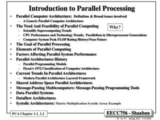
Parallel Computing • Parallel Computing is a central and important problem in many computationally intensive applications, such as image processing, database processing, robotics, and so forth. • Given a problem, the parallel computing is the process of splitting the problem into several subproblems, solving these subproblems simultaneously, and combing the solutions of subproblems to get the solution to the original problem. Introduction to Parallel Processing
Parallel Computer Structures • Pipelined Computers : a pipeline computer performs overlapped computations to exploit temporal parallelism. • Array Processors : an array processor uses multiple synchronized arithmetic logic units to achieve spatial parallelism. • Multiprocessor Systems : a multiprocessor system achieves asynchronous parallelism through a set of interactive processors. Introduction to Parallel Processing
Pipeline Computers • Normally, four major steps to execute an instruction: • Instruction Fetch (IF) • Instruction Decoding (ID) • Operand Fetch (OF) • Execution (EX) Introduction to Parallel Processing
Nonpipelined Processor Introduction to Parallel Processing
Pipeline Processor Introduction to Parallel Processing
Array Computers • An array processor is a synchronous parallel computer with multiple arithmetic logic units, called processing elements (PE), that can operate in parallel. • The PEs are synchronized to perform the same function at the same time. • Only a few array computers are designed primarily for numerical computation, while the others are for research purposes. Introduction to Parallel Processing
Functional structure of array computer Introduction to Parallel Processing
Multiprocessor Systems • A multiprocessor system is a single computer that includes multiple processors (computer modules). • Processors may communicate and cooperate at different levels in solving a given problem. • The communication may occur by sending messages from one processor to the other or by sharing a common memory. • A multiprocessor system is controlled by one operating system which provides interaction between processors and their programs at the process, data set, and data element levels. Introduction to Parallel Processing
Functional structure of multiprocessor system Introduction to Parallel Processing
Multicomputers • There is a group of processors, in which each of the processors has sufficient amount of local memory. • The communication between the processors is through messages. • There is neither a common memory nor a common clock. • This is also called distributed processing. Introduction to Parallel Processing
Grid Computing • Grid Computing enables geographically dispersed computers or computing clusters to dynamically and virtually share applications, data, and computational resources. • It uses standard TCP/IP networks to provide transparent access to technical computing services wherever capacity is available, transforming technical computing into an information utility that is available across a department or organization. Introduction to Parallel Processing
Multiplicity of Instruction-Data Streams • In general, digital computers may be classified into four categories, according to the multiplicity of instruction and data streams. • An instruction stream is a sequence of instructions as executed by the machine. • A data stream is a sequence of data including input, partial, or temporary results, called for by the instruction stream. • Flynn’s four machine organizations : SISD, SIMD, MISD, MIMD. Introduction to Parallel Processing
SISD • Single Instruction stream-Single Data stream • Instructions are executed sequentially but may be overlapped in their execution stages (pipelining). Introduction to Parallel Processing
SIMD • Single Instruction stream-Multiple Data stream • There are multiple PEs supervised by the same control unit. Introduction to Parallel Processing
MISD • Multiple Instruction stream-Single Data stream • The results (output) of one processor may become the input of the next processor in the macropipe. • No real embodiment of this class exists. Introduction to Parallel Processing
MIMD • Multiple Instruction stream-Multiple Data stream • Most Multiprocessor systems and Multicomputer systems can be classified in this category. Introduction to Parallel Processing
Shared-Memory Multiprocessors • Tightly-Coupled MIMD architectures shared memory among its processors. • Interconnected architecture: • Bus-connected architecture – the processors, parallel memories, network interfaces, and device controllers are tied to the same connection bus. • Directly connect architecture – the processors are connected directly to the high-end mainframes. Introduction to Parallel Processing
Distributed-Memory Multiprocessors • Loosely coupled MIMD architectures have distributed local memories attached to multiple processor nodes. • Message passing is the major communication method among the processor. • Most multiprocessors are designed to be scalable in performance. Introduction to Parallel Processing
Network Topologies • Let’s assume processors function independently and communicate with each other. For these communications, the processors must be connected using physical links. Such a model is called a network model or direct-connection machine. • Network topologies: • Complete Graph (Fully Connected Network) • Hypercubes • Mesh Network • Pyramid Network • Star Graphs Introduction to Parallel Processing
Complete Graph • Complete graph is a fully connected network. • The distance between any two processor (or processing nodes) is always 1. • If complete graph network with n nodes, each node has degree n-1. • An example of n = 5: Introduction to Parallel Processing
Hypercubes (k-cube) • A k-cube is a k-regular graph with 2k nodes which are labeled by the k-bits binary numbers. • A k-regular graph is a graph in which each node has degree k. • The distance between two nodes a = (a1a2…ak) and b = (b1b2…bk) is the number of bits in which a and b differ. If two nodes is adjacent to each other, their distance is 1 (only 1 bit differ.) • If a hypercube with n nodes (n = 2k), the longest distance between any two nodes is log2n (=k). Introduction to Parallel Processing
0 1 00 01 10 11 1100 1101 0100 0101 100 101 1001 0000 000 001 1000 0001 0110 0111 1110 1111 110 111 1010 1011 0010 0011 010 011 Hypercube Structures k = 1 k = 2 k = 4 k = 3 Introduction to Parallel Processing
Mesh Network • The arrangement of processors in the form of a grid is called a mesh network. • A 2-dimensional mesh: • A k-dimensional mesh is a set of (k-1) dimensional meshes with corresponding processor communications. Introduction to Parallel Processing
3-Dimensional Mesh A 3-d mesh with 4 copies of 44 2-d meshes Introduction to Parallel Processing
Pyramid Network • A pyramid network is constructed similar to a rooted tree. The root contains one processor. • At the next level there are four processors in the form of a 2-dimensional mesh and all the four are children of the root. • All the nodes at the same level are connected in the form of a 2-dimensional mesh. • Each nonleaf node has four children nodes at the next level. • The longest distance between any two nodes is 2height of the tree. Introduction to Parallel Processing
Pyramid Network Structure A pyramid of height 2 Introduction to Parallel Processing
Star Graphs • k-star graph, consider the permutation with k symbols. • There are n nodes, if there are n (=k!) permutations. • Any two nodes are adjacent, if and only if their corresponding permutations differ only in the leftmost and in any one other position. • A k-star graph can be considered as a connection of k copies of (k-1)-star graphs. Introduction to Parallel Processing
P5 = (3, 2, 1) P0 = (1, 2, 3) P3 = (2, 3, 1) P2 = (2, 1, 3) P1 = (1, 3, 2) P4 = (3, 1, 2) A 3-Star Graph • k=3, there are 6 permutations: What degree of each node for 4-star graph? Introduction to Parallel Processing