Download
1 / 40
410 likes | 745 Vues
Volatility and Hedging Errors. Jim Gatheral September, 25 1999. Background. Derivative portfolio bookrunners often complain that hedging at market-implied volatilities is sub-optimal relative to hedging at their best guess of future volatility but

E N D
Volatility and Hedging Errors Jim Gatheral September, 25 1999
Background • Derivative portfolio bookrunners often complain that • hedging at market-implied volatilities is sub-optimal relative to hedging at their best guess of future volatility but • they are forced into hedging at market implied volatilities to minimise mark-to-market P&L volatility. • All practitioners recognise that the assumptions behind fixed or swimming delta choices are wrong in some sense. Nevertheless, the magnitude of the impact of this delta choice may be surprising. • Given the P&L impact of these choices, it would be nice to be able to avoid figuring out how to delta hedge. Is there a way of avoiding the problem?
An Idealised Model • To get intuition about hedging options at the wrong volatility, we consider two particular sample paths for the stock price, both of which have realised volatility = 20% • a whipsaw path where the stock price moves up and down by 1.25% every day • a sine curve designed to mimic a trending market
Whipsaw and Sine Curve Scenarios 2 Paths with Volatility=20% Spot 4.5 4 3.5 3 2.5 2 1.5 1 0.5 Days 0 0 16 32 48 64 80 96 112 128 144 160 176 192 208 224 240 256
Whipsaw vs Sine Curve: Results P&L vs Hedge Vol. Whipsaw 60,000,000 40,000,000 20,000,000 Hedge Volatility - P&L 10% 15% 25% 40% 20% 30% 35% (20,000,000) (40,000,000) (60,000,000) Sine Wave (80,000,000)
Conclusions from this Experiment • If you knew the realised volatility in advance, you would definitely hedge at that volatility because the hedging error at that volatility would be zero. • In practice of course, you don’t know what the realised volatility will be. The performance of your hedge depends not only on whether the realised volatility is higher or lower than your estimate but also on whether the market is range bound or trending.
Analysis of the P&L Graph • If the market is range bound, hedging a short option position at a lower vol. hurts because you are getting continuously whipsawed. On the other hand, if you hedge at very high vol., and market is range bound, your gamma is very low and your hedging losses are minimised. • If the market is trending, you are hurt if you hedge at a higher vol. because your hedge reacts too slowly to the trend. If you hedge at low vol. , the hedge ratio gets higher faster as you go in the money minimising hedging losses.
Another Simple Hedging Experiment • In order to study the effect of changing hedge volatility, we consider the following simple portfolio: • short $1bn notional of 1 year ATM European calls • long a one year volatility swap to cancel the vega of the calls at inception. • This is (almost) equivalent to having sold a one year option whose price is determined ex-post based on the actual volatility realised over the hedging period. • Any P&L generated by this hedging strategy is pure hedging error. That is, we eliminate any P&L due to volatility movements.
Historical Sample Paths • In order to preempt criticism that our sample paths are too unrealistic, we take real historical FTSE data from two distinct historical periods: one where the market was locked in a trend and one where the market was range bound. • For the range bound scenario, we consider the period from April 1991 to April 1992 • For the trending scenario, we consider the period from October 1996 to October 1997 • In both scenarios, the realised volatility was around 12%
FTSE 100 since 1985 Trend Range
Range ScenarioFTSE from 4/1/91 to 3/31/92 3000 2900 2800 2700 Realised Volatility 12.17% 2600 2500 2400 2300 2200 2100 2000 3/3/91 4/22/91 6/11/91 7/31/91 9/19/91 11/8/91 12/28/91 2/16/92 4/6/92 5/26/92
Trend ScenarioFTSE from 11/1/96 to 10/31/97 Realised Volatility 12.45%
P&L vs Hedge Volatility Range Scenario Trend Scenario
Discussion of P&L Sensitivities • The sensitivity of the P&L to hedge volatility did depend on the scenario just as we would have expected from the idealised experiment. • In the range scenario, the lower the hedge volatility, the lower the P&L consistent with the whipsaw case. • In the trend scenario, the lower the hedge volatility, the higher the P&L consistent with the sine curve case. • In each scenario, the sensitivity of the P&L to hedging at a volatility which was wrong by 10 volatility points was around $20mm for a $1bn position.
Questions? • Suppose you sell an option at a volatility higher than 12% and hedge at some other volatility. If realised volatility is 12%, do you make money? • Not necessarily. It is easy to find scenarios where you lose money. • Suppose you sell an option at some implied volatility and hedge at the same volatility. If realised volatility is 12%, when do you make money? • In the two scenarios analysed, if the option is sold and hedged at a volatility greater than the realised volatility, the trade makes money. This conforms to traders’ intuition. • Later, we will show that even this is not always true.
P&L from Selling and Hedging at the Same Volatility Range Scenario Trend Scenario
Delta Sensitivities • Let’s now see what effect hedging at the wrong volatility has on the delta. • We look at the difference between $-delta computed at 20% volatility and $-delta computed at 12% volatility as a function of time. • In the range scenario, the difference between the deltas persists throughout the hedging period because both gamma and vega remain significant throughout. • On the other hand, in the trend scenario, as gamma and vega decrease, the difference between the deltas also decreases.
Fixed and Swimming Delta • Fixed (sticky strike) delta assumes that the Black-Scholes implied volatility for a particular strike and expiration is constant. Then • Swimming (or floating) delta assumes that the at-the-money Black-Scholes implied volatility is constant. More precisely, we assume that implied volatility is a function of relative strike only. Then
An Aside: The Volatility Skew Volatility Strike
Observations on the Volatility Skew • Note how beautiful the raw data looks; there is a very well-defined pattern of implied volatilities. • When implied volatility is plotted against , all of the skew curves have roughly the same shape.
How Big are the Delta Differences? • We assume a skew of the form • From the following two graphs, we see that the typical difference in delta between fixed and swimming assumptions is around $100mm. The error in hedge volatility would need to be around 8 points to give rise to a similar difference. • In the range scenario, the difference between the deltas persists throughout the hedging period because both gamma and vega remain significant throughout. • On the other hand, in the trend scenario, as gamma and vega decrease, the difference between the deltas also decreases.
Summary of Empirical Results • Delta hedging always gives rise to hedging errors because we cannot predict realised volatility. • The result of hedging at too high or too low a volatility depends on the precise path followed by the underlying price. • The effect of hedging at the wrong volatility is of the same order of magnitude as the effect of hedging using swimming rather than fixed delta. • Figuring out which delta to use at least as important than guessing future volatility correctly and probably more important!
Some Theory • Consider a European call option struck at K expiring at time T and denote the value of this option at time t according to the Black-Scholes formula by . In particular, . • We assume that the stock price S satisfies a SDE of the form where may itself be stochastic. • Path-by-path, we have
where the forward variance . So, if we delta hedge using the Black-Scholes (fixed) delta, the outcome of the hedging process is:
In the Black-Scholes limit, with deterministic volatility, delta-hedging works path-by-path because • In reality, we see that the outcome depends both on gamma and the difference between realised and hedge volatilities. • If gamma is high when volatility is low and/or gamma is low when volatility is high you will make money and vice versa. • Now, we are in a position to provide a counterexample to trader intuition: • Consider the particular path shown in the following slide: • The realised volatility is 12.45% but volatility is close to zero when gamma is low and high when gamma is high. • The higher the hedge volatility, the lower the hedge P&L. • In this case, if you price and hedge a short option position at a volatility lower than 18%, you lose money.
Cooked Scenario: P&L from Selling and Hedging at the Same Volatility
Conclusions • Delta-hedging is so uncertain that we must delta-hedge as little as possible and what delta-hedging we do must be optimised. • To minimise the need to delta-hedge, we must find a static hedge that minimises gamma path-by-path. For example, Avellaneda et al. have derived such static hedges by penalising gamma path-by-path. • The question of what delta is optimal to use is still open. Traders like fixed and swimming delta. Quants prefer market-implied delta - the delta obtained by assuming that the local volatility surface is fixed.
Another Digression: Local Volatility • We assume a process of the form: with a deterministic function of stock price and time. • Local volatilities can be computed from market prices of options using • Market-implied delta assumes that the local volatility surface stays fixed through time.
We can extend the previous analysis to local volatility. So, if we delta hedge using the market-implied delta ,the outcome of the hedging process is:
Define Then If the claim being hedged is path-dependent then is also path-dependent. Otherwise all the can be determined at inception. Writing the last equation out in full, for two local volatility surfaces we get Then, the functional derivative
In practice, we can set by bucket hedging. Note in particular that European options have all their sensitivity to local volatility in one bucket - at strike and expiration. Then by buying and selling European options, we can cancel the risk-neutral expectation of gamma over the life of the option being hedged - a static hedge. This is not the same as cancelling gamma path-by-path. If you do this, you still need to choose a delta to hedge the remaining risk. In practice, whether fixed, swimming or market-implied delta is chosen, the parameters used to compute these are re-estimated daily from a new implied volatility surface. Dumas, Fleming and Whaley point out that the local volatility surface is very unstable over time so again, it’s not obvious which delta is optimal.
Outstanding Research Questions • Is there an optimal choice of delta which depends only on observable asset prices? • How should we price • Path-dependent options? • Forward starting options? • Compound options? • Volatility swaps?
Some References • Avellaneda, M., and A. Parás. Managing the volatility risk of portfolios of derivative securities: the Lagrangian Uncertain Volatility Model. Applied Mathematical Finance, 3, 21-52 (1996) • Blacher, G. A new approach for understanding the impact of volatility on option prices. RISK 98 Conference Handout. • Derman, E. Regimes of volatility. RISK April, 55-59 (1999) • Dumas, B., J. Fleming, and R.E. Whaley. Implied volatility functions: empirical tests. The Journal of Finance Vol. LIII, No. 6, December 1998. • Gupta, A. On neutral ground. RISK July, 37-41 (1997)