Download
1 / 26
270 likes | 550 Vues
Adversarial Search. Chapter 6. History. Much of the work in this area has been motivated by playing chess, which has always been known as a "thinking person's game".

E N D
Adversarial Search Chapter 6
History • Much of the work in this area has been motivated by playing chess, which has always been known as a "thinking person's game". • The history of computer chess goes way back. Claude Shannon, the father of information theory, originated many of the ideas in a 1949 paper. • Shortly after, Alan Turing did a hand simulation of a program to play checkers, based on some of these ideas. • The first programs to play real chess didn't arrive until almost ten years later, and it wasn't until Greenblatt's MacHack 6, 1966 that a computer chess program defeated a good player. • Slow and steady progress eventually led to the defeat of reigning world champion Garry Kasparov against IBM's Deep Blue in May 1997.
Games as Search • Game playing programs are another application of search. • States are the board positions (and the player whose turn it is to move). • Actions are the legal moves. • Goal states are the winning positions. • A scoring function assigns values to states and also serves as a kind of heuristic function. • The game tree (defined by the states and actions) is like the search tree in a typical search and it encodes all possible games. • There are a few key differences, however. • For one thing, we are not looking for a path through the game tree, since that is going to depend on what moves the opponent makes. • All we can do is choose the best move to make next.
Move generation – details Let's look at the game tree in more detail. • Some board position represents the initial state and suppose it's now our turn. • We generate the children of this position by making all of the legal moves available to us. • Then, we consider the moves that our opponent can make to generate the descendants of each of these positions, etc. • Note that these trees are enormous and cannot be explicitly represented in their entirety for any complex game.
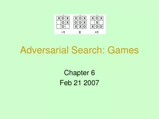
Partial Game Tree for Tic-Tac-Toe Here's a little piece of the game tree for Tic-Tac-Toe, starting from an empty board. Note that even for this trivial game, the search tree is quite big.
Scoring Function • A crucial component of any game playing program is the scoring function. This function assigns a numerical value to a board position. • We can think of this value as capturing the likelihood of winning from that position. • Since in these games one person's win is another's person loss, we will use the same scoring function for both players, simply negating the values to represent the opponent's scores.
Static evaluations • For chess, we typically use linear weighted sum of features Eval(s) = w1 f1(s) + w2 f2(s) + … + wn fn(s) • e.g., w1 = 9 with f1(s) = (number of white queens) – (number of black queens), etc.
Limited look ahead + scoring • The key idea that underlies game playing programs (presented in Shannon's 1949 paper) is that of limited look-ahead combined with the Min-Max algorithm. • Let's imagine that we are going to look ahead in the game-tree to a depth of 2 • (or 2 ply as it is called in the literature on game playing). • We can use our scoring function to see what the values are at the leaves of this tree. These are called the "static evaluations." • What we want is to compute a value for each of the nodes above this one in the tree by "backing up" these static evaluations in the tree. • The player who is building the tree is trying to maximize his score. However, we assume that the opponent (who values board positions using the same static evaluation function) is trying to minimize the score. • So, each layer of the tree can be classified into either a maximizing layer or a minimizing layer.
Example • In this example, the layer right above the leaves is a minimizing layer, so we assign to each node in that layer the minimum score of any of its children. • At the next layer up, we're maximizing so we pick the maximum of the scores available to us, that is, 7. • So, this analysis tells us that we should pick the move that gives us the best guaranteed score, independent of what our opponent does. This is the MIN-MAX algorithm.
Min-Max Here is pseudo-code that implements Min-Max. As you can see, it is a simple recursive alternation of maximization and minimization at each layer. We assume that we count the depth value down from the max depth so that when we reach a depth of 0, we apply our static evaluation to the board. // initial call is MAX-VALUE (state, max-depth) MAX-VALUE (state, depth) if (depth==0) return EVAL (state) v=- for each s in SUCCESSORS (state) do v = MAX (v, MIN-VALUE (s, depth-1)) return v MIN-VALUE (state, depth) if (depth==0) return EVAL (state) v= for each s in SUCCESSORS (state) do v = MIN (v, MAX-VALUE (s, depth-1)) return v
The key idea is that the more lookahead we can do, that is, the deeper in the tree we can look, the better our evaluation of a position will be, even with a simple evaluation function. • In some sense, if we could look all the way to the end of the game, all we would need is an evaluation function that was 1 when we won and -1 then the opponent won. • The truly remarkable thing is how well this idea works. If you plot how deep computer programs can search chess game trees versus their ranking, we see a graph that looks something like this. • The earliest serious chess program (MacHack6), which had a ranking of 1200, searched on average to a depth of 4. • Belle, which was one of the first hardware-assisted chess programs doubled the depth and gained about 800 points in ranking. • Deep Blue, which searched to an average depth of about 13 beat the world champion with a ranking of about 2900.
Brute force? • At some level, the previous is a depressing picture, since it seems to suggest that brute-force search is all that matters. • And Deep Blue is brute indeed... • It had 256 specialized chess processors coupled into a 32 node supercomputer. • It examined around 30 billion moves per minute. • The typical search depth was 13-ply, but in some dynamic situations it could go as deep as 30.
alpha-beta pruning • There's one other idea that has played a crucial role in the development of computer game-playing programs. • It is really only an optimization of Min-Max search, but it is such a powerful and important optimization that it deserves to be understood in detail. • The technique is called alpha-beta pruning, from the Greek letters traditionally used to represent the lower and upper bound on the score.
Suppose that we have evaluated the sub-tree on the left (whose leaves have values 2 and 7). • Since this is a minimizing level, we choose the value 2. So, the maximizing player at the top of the tree knows at this point that he can guarantee a score of at least 2 by choosing the move on the left. • Now, we proceed to look at the subtree on the right. Once we look at the leftmost leaf of that subtree and see a 1, we know that if the maximizing player makes the move to the right then the minimizing player can force him into a position that is worth no more than 1. • Now, we already know that this move is worse than the one to the left, so why bother looking any further? • In fact, it may be that this unknown position is a great one for the maximizer, but then the minimizer would never choose it. So, no matter what happens at that leaf, the maximizer's choice will not be affected.
alpha-beta pruning algorithm • We start out with the range of possible scores (as defined by alpha and beta) going from minus infinity to plus infinity. • alpha represents the lower bound and beta the upper bound. • We call Max-Value with the current board state. • If we are at a leaf, we return the static value. • Otherwise, we look at each of the successors of this state (by applying the legal move function) and for each successor, we call the minimizer (Min-Value) and we keep track of the maximum value returned in alpha. • If the value of alpha (the lower bound on the score) ever gets to be greater or equal to beta (the upper bound) then we know that we don't need to keep looking - this is called a cutoff - and we return alpha immediately. • Otherwise we return alpha at the end of the loop. • The Min-Value is completely symmetric.
alpha-beta // is the best score for MAX, is the best score for MIN // initial call is MAX-VALUE (state, -, , MAX_DEPTH) MAX-VALUE (state, , , depth) if (depth == 0) return EVAL(state) for each s in SUCCESSORS(state) do = MAX (, MIN-VALUE (state, , , depth-1)) if return // cutoff return MIN-VALUE (state, , , depth) if (depth == 0) return EVAL(state) for each s in SUCCESSORS(state) do = MIN (, MAX-VALUE (state, , , depth-1)) if return // cutoff return
We start with an initial call to Max-Value with the initial infinite values of alpha and beta, meaning that we know nothing about what the score is going to be. Max-Value now calls Min-Value on the left successor with the same values of alpha and beta. Min-Value now calls Max-Value on its leftmost successor.
Max-Value is at the leftmost leaf, whose static value is 2 and so it returns that. This first value, since it is less than infinity, becomes the new value of beta in Min-Value. So, now we call Max-Value with the next successor, which is also a leaf whose value is 7. 7 is not less than 2 and so the final value of beta is 2 for this node.
Min-Value now returns this value to its caller. The calling Max-Value now sets alpha to this value, since it is bigger than minus infinity. Note that the range of [alphabeta] says that the score will be greater or equal to 2 (and less than infinity).
Max-Value now calls Min-Value on the right successor with the updated range of [alpha beta].
Min-Value calls Max-Value on the left leaf and it returns a value of 1.
This is used to update beta in Min-Value, since it is less than infinity. Note that at this point we have a range where alpha (2) is greater than beta (1). This situation signals a cutoff in Min-Value and it returns beta (1), without looking at the right leaf. So, a total of 3 static evaluations were needed instead of the 4 we would have needed under pure Min-Max.
alpha-beta pruning There are a couple of key points to remember about - pruning: • It is guaranteed to return exactly the same value as the Min-Max algorithm. It is a pure optimization without any approximations or tradeoffs. • In a perfectly ordered tree, with the best moves on the left, alpha beta reduces the cost of the search from order bd to order b(d/2), that is, we can search twice as deep! • We already saw the enormous impact of deeper search on performance… • Now, this analysis is optimistic, since if we could order moves perfectly, we would not need alpha-beta. But, in practice, performance is close to the optimistic limit.
Practical matters • Chess and other such games have incredibly large trees with highly variable branching factor (especially since alpha-beta cutoffs affect the actual branching of the search). • If we picked a fixed depth to search, as we've suggested earlier, then much of the time we would finish too quickly and at other times take too long. • A better approach is to use iterative deepening and thus always have a move ready and then simply stop after some allotted time.
Games in practice • Checkers: Chinook ended 40-year-reign of human world champion Marion Tinsley in 1994. Used a precomputed endgame database defining perfect play for all positions involving 8 or fewer pieces on the board, a total of 444 billion positions. • Chess: Deep Blue defeated human world champion Garry Kasparov in a six-game match in 1997. Deep Blue searches 200 million positions per second, uses very sophisticated evaluation, and undisclosed methods for extending some lines of search up to 40 ply. • Othello: human champions refuse to compete against computers, who are too good. • Go: human champions refuse to compete against computers, who are too bad. In go, b > 300, so most programs use pattern knowledge bases to suggest plausible moves.