Download
1 / 27
270 likes | 701 Vues
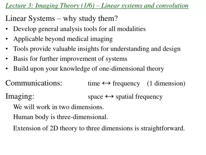
Lecture 3: Imaging Theory (1/6) – Linear systems and convolution. Linear Systems – why study them? Develop general analysis tools for all modalities Applicable beyond medical imaging Tools provide valuable insights for understanding and design Basis for further improvement of systems

E N D
Lecture 3: Imaging Theory (1/6) – Linear systems and convolution Linear Systems – why study them? • Develop general analysis tools for all modalities • Applicable beyond medical imaging • Tools provide valuable insights for understanding and design • Basis for further improvement of systems • Build upon your knowledge of one-dimensional theory Communications: time ↔ frequency (1 dimension) Imaging: space ↔ spatial frequency We will work in two dimensions. Human body is three-dimensional. Extension of 2D theory to three dimensions is straightforward.
Linearity Conditions Let f1(x,y) and f2(x,y) describe two objects we want to image. f1(x,y) can be any object and represent any characteristic of the object. (e.g. color, intensity, temperature, texture, X-ray absorption, etc.) Assume each is imaged by some imaging device (system). Let f1(x,y) → g1(x,y) f2(x,y) → g2(x,y) Let’s scale each object and combine them to form a new object. a f1(x,y) + b f2(x,y) What is the output? If the system is linear, output is a g1(x,y) + b g2(x,y)
Linearity Example: Is this a linear system?
Linearity Example: Is this a linear system? 9 → 3 16→ 4 9 + 16 = 25 → 5 3 + 4 ≠ 5 Not linear.
Example in medical imaging: Analog to digital converter Doubling the X-ray photons → doubles those transmitted Doubling the nuclear medicine → doubles the reception source energy MR: Maximum output voltage is 4 V. Now double the water: The A/D converter system is non-linear after 4 mV. (overranging)
Linearity allows decomposition of functions Linearity allows us to decompose our input into smaller, elementary objects. Output is the sum of the system’s response to these basic objects. Elementary Function: The two-dimensional delta function δ(x,y) δ(x,y) has infinitesimal width and infinite amplitude. Key: Volume under function is 1. δ(x,y)
The delta function as a limit of another function Powerful to express δ(x,y) as the limit of a function A note on notation: Π(x) = rect(x) Gaussian: lim a2 exp[- a2(x2+y2)] =δ(x,y) 2D Rect Function: lim a2 Π(ax)Π(ay) = δ(x,y) where Π(x) = 1 for |x| < ½ For this reason, δ(bx) = (1/|b|) δ(x)
Sifting property of the delta function The delta function at x1 = ε, y1= η has sifted out f (x1,y1) at that point. One can view f (x1,y1) as a collection of delta functions, each weighted by f (ε,η).
From previous page, Imaging Analyzed with System Operators Let system operator (imaging modality) be , so that Why the new coordinate system (x2,y2)?
From previous page, Imaging Analyzed with System Operators Let system operator (imaging modality) be , so that Then, Generally System operating on entire blurred object input object g1 (x1,y1) By linearity, we can consider the output as a sum of the outputs from all the weighted elementary delta functions. Then,
System response to a two-dimensional delta function Output at (x2 , y2) depends on input location (ε,η). Substituting this into yields the Superposition Integral
Example in medical imaging: Consider a nuclear study of a liver with a tumor point source at x1= ε, y1= η Radiation is detected at the detector plane. To obtain a general result, we need to know all combinations h(x2, y2; ε,η ) By “general result”, we mean that we could calculate the image I(x2, y2) for any source input S(x1, y1)
Time invariance A system is time invariant if its output depends only on relative time of the input, not absolute time. To test if this quality exists for a system, delay the input by t0. If the output shifts by the same amount, the system is time invariant i.e. f(t)→ g(t) f(t - to) → g(t - to) input delay output delay Is f(t)→ f(at) → g(t) (an audio compressor) time invariant?
Time invariance A system is time invariant if its output depends only on relative time of the input, not absolute time. To test if this quality exists for a system, delay the input by t0. If the output shifts by the same amount, the system is time invariant i.e. f(t)→ g(t) f(t - to) → g(t - to) input delay output delay Is f(t)→ f(at) → g(t) (an audio compressor) time invariant? f(t - to) → f(at) → f(a(t – to)) - output of audio compressor f(at – to) - shifted version of output (this would be a time invariant system.) So f(t)→ f(at) = g(t) is not time invariant.
Space or shift invariance A system is space (or shift) invariant if its output depends only on relative position of the input, not absolute position. If you shift input → The response shifts, but in the plane, the shape of the response stays the same. If the system is shift invariant, h(x2, y2; ε,η ) = h(x2-ε , y2-η) and the superposition integral becomes the 2D convolution function: Notation: g = f**h (** sometimes implies two-dimensional convolution, as opposed to g = f*h for one dimension. Often we will use * with 2D and 3D functions and imply 2D or 3D convolution.)
One-dimensional convolution example: g(x) = Π(x)*Π(x/2) Recall: Π(x) = 1 for |x| < ½ Π(x/2) = 1 for |x|/2 < ½ or |x| < 1 Flip one object and drag across the other. flip delay
One-dimensional convolution example, continued: Case 1: no overlap of Π(x-x’) and Π(x’/2) Case 2: partial overlap of Π(x-x’) and Π(x’/2)
One-dimensional convolution example, continued(2): Case 3: complete overlap Case 4: partial overlap Case 5: no overlap
One-dimensional convolution example, continued(3): Result of convolution:
Two-dimensional convolution sliding of flipped object
2D Convolution of letter E - circle vs. square. E ** square E ** circle