Particle Swarm Optimization Algorithms to Continuous Problem

1. Particle Swarm Optimization Algorithms to Continuous Problem Monday, March 10, 2014 by Yoon-Teck Bau, Hong-Tat Ewe, Chin-Kuan Ho Faculty of Information Technology Multimedia University, Malaysia {ytbau, htewe, ckho}@mmu.edu.my http://pesona.mmu.edu.my/~ytbau/

2. Talk Outlines • Research Objective • Particle Swarm Optimization (PSO) Algorithms Overview • PSO to Continuous Problem • PSO and Non-linear Maximization Problem • Experiments and Results • Conclusions • References

3. Research Objective • To study PSO in continuous problem • To compare the performance of genetic algorithms with PSO in maximization problem • To share and exchange knowledges related to PSO and swarm intelligence

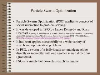
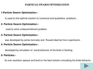
4. PSO Algorithms Overview • Introduced by Russel Ebenhart (an Electrical Engineer) and James Kennedy (a Social Psychologist) in 1995 • Belongs to the categories of Swarm Intelligence techniques and Evolutionary Algorithms for optimization • Inspired by the social behavior of birds, which was studied by Craig Reynolds (a biologist) in late 80s and early 90s • Optimization problem representation is similar to the genes encoding methods used in GAs but for PSO the variables are called dimensions, that create a multi-dimensional hyperspace. • "Particles" fly in this hyperspace and try to find the global minima/maxima, their movement being governed by a simple mathematical equation.

5. pi xt pg xt+1 vt PSO Basic Mathematical Equations • Basic mathematical equations in PSO: particle’s personal best particle’s neighbours best where particle’s itself

6. R1, R2, R3 : random numbers between 0 and 1ω : inertia weight between 0.01 and 0.7 : best position of a particleŷ : best position of a randomly chosen other particle from within the swarmz : a random velocity vectora, b, c : constants Repulsive PSO (1) • RPSO is a global optimization algorithm, belongs to the class of stochastic evolutionary global optimizers, a variant of particle swarm optimization (PSO).

7. Repulsive PSO (2) • The different realizations of PSO, where there is a repulsion between particles that can prevent the swarm being trapped in local minima (which would cause a premature convergence and would lead the optimization algorithm to fail to find the global optimum). • The main difference between PSO and RPSO is the propagation mechanism (vt+1) to determine new positions for a particle in the search space. • RPSO is capable of finding global optima in more complex search spaces. On the other hand, compared to PSO it may be slower on certain types of optimization problems.

8. PSO Pseudocode fori = 1 to number of particles n forj =1 to number of dimensions m C2 = uniform random number C3 = uniform random number V[ i ][ j ] = C1*V[ i ][ j ] + C2*(P[ i ][ j ]-X[ i ][ j ]) + C3*(G[ i ][ j ]-X[ i ][ j ]) X[ i ][ j ] = X[ i ][ j ] + V[ i ][ j ]

9. PSO Algorithms Common Parameter • c1/ω is an inertial constant. Good values are usually slightly less than 1. • c2 and c3 are two random vectors with each component generally a uniform random number between 0 and 1. • Very frequently the value of c1/ω is taken to decrease over time; e.g., one might have the PSO run for a certain number of iterations and decrease linearly from a starting value (0.9, say) to a final value (0.4, say) in order to facilitate exploitation over exploration in later states of the search.

10. PSO to Continuous Problem

11. PSO to Continuous Problem • Continuous optimization problem as opposed to discrete optimization, the variables used in the objective function can assume real values, e.g., values fromintervals of the real line. • The particles "communicate" information they find about each other by updating their velocities in terms of local and global bests; when a new best is found, the particles will change their positions accordingly so that the new information is "broadcast" to the swarm. • The particles are always drawn back both to their own personal best positions and also to the best position of the entire swarm. • They also have stochastic exploration capability via the use of the random multipliers c2, and c3. • Typical convergence conditions include reaching a certain number of iterations, reaching a certain fitness value, and so on.

12. PSO and Non-linear Maximization Problem Non-linear Maximization problem: f(x1,x2,x3) is maximum if 0 <= x1, x2, x3 <= 10 x1 = 10 x2 = 0 x3 = 10 f(x1,x2,x3) = 110

13. Experiments and Results (1) • Both the PSO's and GA's approaches are implemented in Java v6.0 on Pentium4-1.80GHz CPU, 512M RAM, WinXP OS. • GA’s uses roulette wheel selection scheme, elitist model, one point crossover and uniform mutation.

14. Experiments and Results (2) GA’s Parameter PSO’s Parameter

15. Experiments and Results (3) GA’s Best max fitness value = 109.78 Best member: x1 = 9.9931 x2 = 0.0075 x3 = 9.9949 Total time (ms) = 3469 PSO’s Best max fitness value = 110.00 Best member: x1 = 10.0 x2 = 0.0 x3 = 10.0 Total time (ms) = 344 Note: Mean # of iteration = 72.540000 Mean fn val = 110.000000 Std. dev. fn val = 0.000000 Success rate = 100.00%

16. Conclusion • PSO has proven both very effective and quick when applied to a diverse set of optimization problems. • GA’s results can be much better if uniform mutation, MU(x) := U([a,b]), is replaced by a Gaussian mutation, where x [a,b], m is mean, s is variance, andRi is sum of 12 random numbers from the range [0..1]. • In future, it will be interesting to study and to compare the performance of PSO’s with GA’s and also ACO’s to solve discrete type of problem.

17. References • Kennedy J, Eberhart R. C., and Shi Y. (2001). Swarm Intelligence. USA: Academic Press. • Michalewicz Z. (1996). Genetic Algorithms + Data Structures = Evolution Programs. 3rd, Revised and Extended Edition. USA: Springer.