Download
1 / 127
1.31k likes | 1.85k Vues
National Cheng Kung University, Taiwan. The optical carrier before modulation is in the form of a continuous wave (CW) and its electric field can be written as ...

E N D
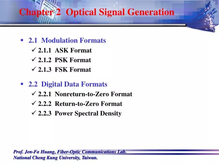
Chapter 2 Optical Signal Generation • 2.1 Modulation Formats • 2.1.1 ASK Format • 2.1.2 PSK Format • 2.1.3 FSK Format • 2.2 Digital Data Formats • 2.2.1 Nonreturn-to-Zero Format • 2.2.2 Return-to-Zero Format • 2.2.3 Power Spectral Density
Chapter 2 Optical Signal Generation • 2.3 Bit-Stream Generation • 2.3.1 NRZ Transmitters • 2.3.2 RZ Transmitters • 2.3.3 Modified RZ Transmitters • 2.3.4 DPSK Transmitters and Receivers • 2.4 Transmitter Design • 2.4.1 Coupling Losses and Output Stability • 2.4.2 Wavelength Stability and Tunability • 2.4.3 Monolithic Integration • 2.4.4 Reliability and Packaging
2.1 Modulation Formats • The optical carrier before modulation is in the form of a continuous wave (CW) and its electric field can be written as where Re denotes the real part, E is the electric field vector, ê is a unit vector representing the state of the polarization of the optical field, A0 is its amplitude, w0 is its carrier frequency, and f0 is its phase. The spatial dependence of E is suppressed for simplicity of notation.
2.1 Modulation Formats • Figure 2.1 shows schematically the time dependence of the modulated optical carrier for the three modulation formats using a specific bit pattern. Figure 2.1: Modulated optical carrier in the case of the ASK, PSK, and FSK formats for a specific bit pattern shown on the top.
2.1 Modulation Formats • Since only the amplitude A0 is modulated in Eq. (2.1.1) in the case of ASK, the electric field associated with the modulated carrier can be written as where A0(t)changes with time in the same fashion as the electrical bit stream. • In the digital case, where P0is the peak power, fp(t)represents the optical pulse shape, Tb = 1/B is thebit slot at the bit rate B, and the random variable b, takes values 0 and 1, dependingon whether the n-th bit in the optical signal corresponds to a 0 or 1.
2.1.1 ASK Formats • In most practical situations, A0 is set to zero during transmission of “0” bits. • The ASK format is also known as the on-off keying (OOK). Most digital lightwave systems employ ASK because its use simplifies the design of optical transmitters and receivers considerably. • The implementation of on-off keying in an optical transmitter requires that the intensity (or the power) of the optical carrier is turned on and off in response to an electrical bit stream.
2.1.1 ASK Formats • The simplest approach makes use of a direct-modulation technique in which the electrical signal is applied directly to the driving circuit of a semiconductor laser or a light-emitting diode. • Typically, the laser is biased slightly below threshold so that it emits no light (except for some spontaneous emission). • During each “1” bit, the laser goes beyond its threshold and emits a pulse whose duration is nearly equal to that of the electrical pulse. • Such an approach works as long as the laser can be turned on and off as fast as the bit rate of the signal to be transmitted.
2.1.1 ASK Formats • The reason is related to phase changes that invariably occur when laser power is changed by modulating the current applied to a semiconductor laser. • Physically,one must inject additional electrons and holes into the active region of the laser. This increase in the charge-carrier density changes the refractive index of the active region slightly and modifies the carrier phase f0 in Eq. (2.1.2) in a time-dependent fashion. • Although such unintentional phase changes are not seen by a photodetector (as it responds only to optical power), they chirp the optical pulse and broaden its spectrum by adding new frequency components.
2.1.1 ASK Formats • Such spectral broadening is undesirable because it can lead to temporal broadening of optical pulses as they propagate through an optical fiber. • For this reason, direct modulation of the laser output becomes impractical as the bit rate of a lightwave system is increased beyond 2.5 Gb/s. • Figure 2.2shows the basic ideaschematically. Two types of external modulators are employed for lightwave systems.
2.1.1 ASK Formats • Figure 2.2: Schematic illustration of the external- modulation scheme. A DFB laser is biased at a constant current while the time-dependent electrical signal is applied to the modulator.
2.1.1 ASK Formats • Figure 2.3 shows an example of each kind. The modulator shown in part (a) makes use of the electro-optic effect through which the refractive index of a suitable material (LiNbO3 in practice) can be changed by applying a voltage across it. • Changes in the refractive index modify the phase of an optical field propagating inside that material. Phase changes are converted into amplitude modulation using a Mach-Zehnder Interferometer (MZI) made of two LiNbO3 waveguides as shown in Figure 2.3(a).
2.1.1 ASK Formats Figure 2.3: Two kinds of external modulators: (a) a LiNbO3 modulator in the Mach-Zehnder configuration; (b) an electro-absorption modulator with multi-quantum-well (MQW) absorbing layers.
2.1.1 ASK Formats • Insertion losses can be reduced significantly (to below 1 dB) by using an electro-absorption modulator shown schematically in Figure 2.3(b). • The reason behind this reduction is that an electro-absorption modulator is made with the same material used for semiconductor lasers, and thus it can be integrated monolithically with the optical source.
2.1.2 PSK Formats • In the case of PSK format, the optical bit stream is generated by modulating the phase f0 in Eq. (2.1.1), while the amplitude A0 and the frequency w0of the optical carrier arekept constant. • The electric field of the optical bit stream can now be written as where the phase f0 changes with time in the same fashion as the electrical bit stream.
2.1.2 PSK Formats • For binary PSK, the phase fm takes two values, commonly chosen to be 0 and p, andit can be written in the form where fp(t)represents the temporal profile and the random variable bntakes values0and 1, depending on whether the n-th bit in the optical signal corresponds to a 0 or 1.
2.1.2 PSK Formats • Figure 2.1 shows the binary PSK format schematically for a specific bit pattern. An interesting aspect of the PSK format is that the optical power remains constant during all bits, and the signal appears to have a CW form. • The only solution is to employ a homodyne or a heterodyne detection technique in which the optical bit stream is combined coherently with the CW output of a local oscillator (a DFB laser) before the signal is detected. • The interference between the two optical fields creates a time-dependent electric current that contains all the information transmitted through PSK.
2.1.2 PSK Formats • This can be seen mathematically by writing the total field incident on the photodetector as (in the complex notation) • where the subscript L denotes the corresponding quantity for the local oscillator. • The current generated at the photodetector is given by Id = Rd|Ed(t)|2, where Rdis theresponsivity of the photodetector.
2.1.2 PSK Formats • It is easy to see that Idvaries with time as • Since Id(t) changes from bit to bit as f0(t) changes, one can reconstruct the original bit stream from this electrical signal. • The PSK format is rarely used in practice for lightwave systems because it requires the phase of the optical carrier to remain stable so that phase information can be extracted at the receiver without ambiguity.
2.1.2 PSK Formats • A variant of the PSK format, known as differential PSK or DPSK, is much morepractical for lightwave systems. • In the case of DPSK, information is coded by using the phase difference between two neighboring bits. For instance, if fkrepresents the phaseof the k-th bit, the phase difference Df = fk - fk-1is changed by0orp, depending onwhether the k-th bit is a “0” or “1”. • The DPSK format does not suffer from the phase-stability problem because information coded in the phase difference between two neighboring bits can be recovered successfully as long as the carrier phase remains stable over a duration of two bits.
2.1.2 PSK Formats • This condition is easily satisfied at bit rates >1 Gb/s because the line width of a DFB laser is typically below 10 MHz, indicating that the carrier phase does not change significantly over a duration of 1 ns or so. • A modulation format that can be useful for enhancing the spectral efficiency of lightwave systems is known as quaternary PSK (QPSK). • In this format, the phase modulator takes two bits at a time and produces one of the four possible phases of the carrier, typically chosen to be 0, p/2, p, and3p/2for bit combinations00, 01, 11, and 10, respectively.
2.1.3 FSK Formats • In the case of FSK modulation, information is coded on the optical carrier by shifting the carrier frequency w0itself [see Eq. (2.1.1)]. • For a binary digital signal, w0 takes two values, say, w0-Dwandw0+Dw, depending on whether a “0” or “1” bit is being transmitted. The shift Df = Dw/2pis called the frequency deviation. • The quantity 2Df is sometimes called tone spacing, asit represents frequency separation between “0”and “1” bits.
2.1.3 FSK Formats • Figure 2.1 shows schematically how the electric field varies in the case of FSK format. Mathematically, it can be written as • where + and - signs correspond to “1” and “0” bits, respectively. • The argument of the exponential function can be written as w0t + (f0±Dwt).The FSK format can also be viewed as a special kind of PSK modulation for which the carrier phase increases or decreases linearly over the bit duration.
2.1.3 FSK Formats • The modulated carrier of FSK has constant power, and the information encoded within the bit stream cannot be recovered through direct detection: One must employ heterodyne detection for decoding an FSK-coded optical bit stream. • In the case of ASK, the frequency shift, or chirping of the emitted optical pulse, is undesirable. But the same frequency shift can be used to advantage for the purpose of FSK. • Typical values of frequency shifts are ~1 GHz/mA.
2.2 Digital Data Formats • The pulse can occupy the entire bit slot or only a part of it, leading to two main choices for the format of optical bit streams. • These two choices are shown in Figure 2.4 and are known as the return-to-zero (RZ) and nonreturn-to-zero (NRZ) formats.
2.2 Digital Data Formats • These two choices are shown in Figure 2.4 and are known as the return-to-zero (RZ) and nonreturn-to-zero (NRZ) formats. • Figure 2.4: Optical bit stream 010110… coded using (a) return-to-zero (RZ) and (b) nonreturn-to-zero (NRZ) formats.
2.2.1 Nonreturn-to-Zero Format • In the NRZ format, the optical pulse representing each 1 bit occupies the entire bit slot. As seen in Figure 2.4(b), the optical field does not drop to zero between two or more successive 1 bits. • The main advantage of the NRZ format is that the bandwidth associated with this format is smaller than that of the RZ format by about a factor of 2. • The reduced bandwidth of an NRZ signal can be understood qualitatively from Figure 2.4(b) by noting that on-off transitions occur much less often for an NRZ signal.
2.2.1 Nonreturn-to-Zero Format • The use of NRZ format for lightwave systems is not always the right choice because of the dispersive and nonlinear effects that can distort optical pulses and spread them outside their assigned bit slot. • Since the pulse occupies the entire bit slot, the NRZ format cannot tolerate even a relatively small amount of pulse broadening and is quite vulnerable to intersymbol crosstalk. • Moreover, a long sequence of “1” or “0” bits contains no information about the bit duration and makes it difficult to extract the clock electronically with a high accuracy.
2.2.2 Return-to-Zero Format • In the RZ format, each optical pulse representing “1” bit is chosen to be shorter than the bit slot, and its amplitude returns to zero before the bit duration is over, as seen in Figure 2.4(a). • In an interesting variant of the RZ format, known as the chirped RZ (CRZ) format, optical pulses in each bit slot are chirped suitably before they are launched into the fiber link. • Its main advantage is that it has a smaller signal bandwidth than the conventional RZ format.
2.2.3 Power Spectral Density • To find the power spectrum of an optical bit stream, we begin with the electric field, E(t)= Re[A(t).exp(-iw0t)], where A(t)is the complex amplitude of the modulated carrier. • In the case of the ASK format, A(t)can be written as • where bnis a random number taking values 0 or 1, Ap(t) represents the pulse shape.
2.2.3 Power Spectral Density • We have introduced b(t) as • where d(t)represents the delta function defined to be zero for all values of t≠0 and normalized such that . • Physically, one can interpret b(t)as the impulse response of a filter.
If we assume that A(t) represents a stationary stochastic process, its power spectral density SA(w)can be found from the Wiener-Khintchine theorem using where GA(t) = <A*(t)A(t+t)> is the autocorrelation function of A(t) and the angle brackets <.> denote ensemble averaging.
2.2.3 Power Spectral Density • It follows from Eqs. (2.2.1) ~ (2.2.3) that where the power spectral density Sb(w)is defined • similar to Eq. (2.2.3) and ~Ap(w) is the Fourier • transform of the pulse amplitude Ap(t) defined as
2.2.3 Power Spectral Density • To find Sb(w), we first calculate the autocorrelation function of b(t)using Gb(t) = <b(t)b(t + t)> . If we use b(t)from Eq. (2.2.2), we obtain • If we replace the ensemble average with a time average over the entire bit stream andmake the substitution n - k = m, Eq. (2.2.6) can be written as where the correlation coefficient rm is defined as
2.2.3 Power Spectral Density • Taking the Fourier transform of Eq. (2.2.7) and substituting that in Eq. (2.2.4), we obtain the power spectral density of an optical bit stream: • The correlation coefficients can be easily calculated by noting that “1” and “0” bits are equally likely to occur in any realistic bit stream. • It is easy to show that when bntakes values 1 or 0 with equal probabilities,
2.2.3 Power Spectral Density • Using these values in Eq. (2.2.11), we obtain • If we use the well-known identity the power spectral density can be written as
2.2.3 Power Spectral Density • We now apply Eq. (2.2.13) to the RZ and NRZ formats. In the case of the NRZ format, each pulse occupies the entire bit slot. • Assuming a rectangular shape, Ap(t)equals (P0)1/2 within the bit slot of duration Tb but becomes zero outside of it. • Taking the Fourier transform of Ap(t), we obtain • where sinc(x) = sin(x)/x is the so-called sinc function. • Substituting the preceding expression in Eq. (2.2.13), we obtain
2.2.3 Power Spectral Density • This spectrum is shown in Figure 2.5(a). The spectrum contains a discrete component at the zero frequency. • Recall that the zero-frequency component of SA(w) is actually located at w0when one considers the spectrum of the electric field. • The continuous part of the spectrum is spread around the carrier in a symmetric fashion. • Most of the spectrum is confined within the bandwidth 2B for an NRZ bit stream at the bit rate B, and the 3-dB bandwidth (full width at half maximum or FWHM) is about B.
2.2.3 Power Spectral Density Figure 2.5: Power spectral density of (a) NRZ bit stream and (b) RZ bit stream with 50% duty cycle. Frequencies are normalized to the bit rate and the discrete part of the spectrum is shown by vertical arrows.
2.2.3 Power Spectral Density • In the case of an RZ bit stream, spectral density depends on the duty cycle of the RZ pulse. • Assuming that each “1” bit occupies a fraction dcof the bit slot and assuming a rectangular shape for the optical pulse, the pulse spectrum is found to be • As expected, this spectrum is wider than that given in Eq. (2.2.14) by a factor of l/dc.
2.2.3 Power Spectral Density • When we substitute Eq. (2.2.16) in Eq. (2.2.13), we notice another important difference. Which ones survive depends on the duty factor. • For example, for a duty cycle of 50% every even component (except m = 0) vanishes but all odd components survive. This case is shown in Figure 2.5(b). • In general, all discrete components can be present in an RZ bit stream depending on the pulse shape and the duty factor used.
2.3 Bit-Stream Generation • The format of choice for most lightwave systems is the ASK format. It can be implemented using both the RZ and NRZ coding schemes. • In an attempt to improve the spectral efficiency of dense WDM systems, several new formats mix the basic RZ scheme with phase modulation.
2.3.1 NRZ Transmitters • The design of an NRZ transmitter is relatively simple since the electrical signal that needs to be transmitted is itself usually in the NRZ format. • It is thus sufficient to use the scheme shown in Figure 2.2, where a single modulator, known as the data modulator, converts the CW light from a DFB semiconductor laser into an optical bit stream in the • NRZ format. • The data modulator can be integrated with the DFB laser if it is based on the electro-absorption effect.
2.3.1 NRZ Transmitters • Figure 2.6 shows schematically the design of a LiNbO3 modulator. • The input CW beam is split into two parts by a 3-dB coupler that are recombined back by another 3-dB coupler after different phase shifts have been imposed on them by applying voltages across two waveguides that form the two arms of the MZI. • To understand this conversion process, we consider the transmission characteristics of such a modulator.
2.3.1 NRZ Transmitters • Figure 2.6: Schematic of a LiNbO3 modulator, The Mach-Zehnder configuration converts the input CW beam into an optical bit stream by applying appropriate voltages across the two arms of the interferometer.
2.3.1 NRZ Transmitters • The outputs Aband Acexiting from the bar and cross ports of an MZ interferometer, can be obtained from the matrix equation • where Aiis the incident field and fj(t)= pVj(t)/Vpis the phase shift in the j-th arm when a voltage Vj is applied across it (j = 1, 2). • Here, Vjis the voltage required to produce a pphase shift; this parameter is typically in the range of 3 to 5 V.
2.3.1 NRZ Transmitters • The transfer function for the bar or cross port is easily obtained from Eq. (2.3.1). • For the cross port, the modulator response is governed by • The phase shift f1 + f2 can be reduced to a constant if we choose voltages in the two arms such that • V2(t) = -V1(t) + Vb , where Vbis a constant bias voltage.
2.3.1 NRZ Transmitters • The power transfer function, or the time-dependent transmissivity of the modulator, takes the form • Note that the transfer function of a MZ modulator is nonlinear in applied voltage V1. • To generate the NRZ bit stream, the modulator is typically biasedat the half-power point by choosing Vb = -Vp/2. • The applied voltage V1(t)is then changed using a bipolar electrical NRZ signal that changes from -Vp/4to +Vp/4 between “0” and “1” bits.
2.3.2 RZ Transmitters • An alternative approach adopts the scheme shown in Figure 2.7. It first generates an NRZ signal using a data modulator and then converts it into an RZ bit stream using a second modulator that is driven by a sinusoidal clock at the bit rate. • The second modulator is sometimes called the “pulse carver” because it splits a long optical pulse representing several “1” bits into multiple pulses, each being shorter than the bit slot. • Three different biasing configurations can be used to create RZ bit streams with duty cycles ranging from 33to 67%.
2.3.2 RZ Transmitters • Figure 2.7: Schematic of an RZ transmitter. The data modulator creates an NRZ signal that is transformed into an RZ bit stream by the second modulator acting as a pulse carver.
2.3.2 RZ Transmitters • For a sinusoidal clock, the transfer function or the transrnissivity of the second modulator becomes • Figure 2.8 shows the clock signal at 40Gb/s together with the RZ pulses obtained with such a clock by plotting Tmas a function of time. The duty cycle of RZ pulses is about 50%. • In practice, duty cycle can be adjusted by reducing the voltage swing and adjusting the bias voltage applied to the modulator, or using a third modulator.