Download
1 / 22
220 likes | 561 Vues
Science Case for ALPACA. Arlin Crotts (Columbia University) for the LAMA Collaboration. . Proto-ALPACA imaging focal plane. 0.86 deg diameter field 6 CCDs, 7 arcmin square, 2048x2048 E2V 1 CCD for u,b,i,z; 2 r CCDs

E N D
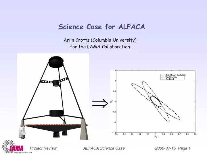
Project ReviewALPACA Science Case 2005-07-15 Page 1 Science Case for ALPACA Arlin Crotts (Columbia University) for the LAMA Collaboration
Project ReviewALPACA Science Case 2005-07-15 Page 2 Proto-ALPACA imaging focal plane • 0.86 deg diameter field • 6 CCDs, 7 arcmin square, 2048x2048 E2V • 1 CCD for u,b,i,z; 2 r CCDs • NASA NEOs: add two rows (6 CCDs total) for near-Earth asteroids (plus weak lensing, bulge microlensing, LSS, variable stars, etc.) full ALPACA imaging focal plane 3 deg diameter field 240 CCDs, 8 arcmin square, 2048x2048 Fairchild deep strip, 8 columns with 6 rows of u, 4 b, and 2 each r, i, z wide strip, 8 more columns with 4 u, and 2 each b, r, i, z NEO “ears”: 4 more columns of 2 each of r, i
Project ReviewALPACA Science Case 2005-07-15 Page 3 ALPACASurveyProducts(P. 1) • Well-sampled, 5-band SN light curves (to r ~ 25 each night) to discover and identify ~50000 SNe Ia and ~12000 SN Iab/II per year. SNe Ia mostly over 0.2 < z < 0.8 range, which is ideal for detailing the evolution and dynamics of dark energy • WeakLensing: 700square degrees with multiband data good for photometric z’s • Galaxyphotometricredshiftsampletor ~ 28;roughly1billiongalaxies • Forgalaxyclusters, shouldachievesamerichnessasSDSSclustercatalog(toz = 0.3)buttoz = 1.Sampleof~30000clusters • Includes strongQSOlensinge.g.,J12514-2914. • MapofSculptor supercluster (z = 0.11). Novae, bright variables. • Should find several orphan GRB afterglows per year.
Project ReviewALPACA Science Case 2005-07-15 Page 4 ALPACASurveyProducts(cont.) • Monitor 100,000s of AGNe to r ~ 26 for multiband variability. • Large scale structure over 4 Gpc3 (comoving) to z = 1 and 9 Gpc3 to z = 1.5. • Includes M83 (7 Mpc away, starburst); two Seyferts: NGC 2997 (17 Mpc), NGC 1097 (17 Mpc). Follow cepheids, miras, novae, eclipsing variables. • Passes through Galactic Nucleus; will find >5000 Bulge microlensing events per year; superlative extrasolar planet search resource. • Many 1000s of variable stars: Galactic structure. • Huge variety of stellar surveys. • Discover ~50 Kuiper Belt objects per night. • Trace near-Earth asteroids of 1 km diameter to Jupiter’s orbit, reconstruct orbits well within 1 AU and detect 50 m objects at 1 AU.
ALPACA and Near-Earth Objects • Proto-ALPACA (with NEO extension) will be able to detect (and recover) NEOs down to 100m diameter at 1AU and 1km at 5AU, for albedo a=0.05. (ALPACA will reach 50m and 500m, respectively.) • NASA’s goal is to find 90% of all NEOs with diameter > 1km by year 2008 (for which they will be late), but observations concentrate on low ecliptic latitude . (Proto-)ALPACA covers –6 < < -53 deg. • Proto-ALPACA will have figure-of-merit A (efficiency x area x solid angle) larger than any competitor soon (including first-generation PanSTARRS), and ALPACA will have larger A than any planned survey (including LSTT). • (Proto-)ALPACA filter bands are tuned to separate comets from common asteroid types. • (Proto-)ALPACA will find unprecedented number of Kuiper-belt objects, as well. Density on sky (in ecliptic coordinates) of asteroids weighted by Earth impact hazard (contours increase proportional to density), from Kaiser et al. 2001. Project ReviewALPACA Science Case 2005-07-15 Page 5
ALPACA for Bulge Microlensing • OGLE III has 1.3m telescope with a 0.34 deg2 FOV, covers 90 deg2 total, spending ~60s/night per pointing, finds about 500 microlensing events per year. • Proto-ALPACA will spend ~160s per star, but has collecting area 35 times greater -> will go 10x deeper -> 30x(density of stars). Will cover 5 deg2 -> 1000 events per year (3000/year w/ NEO). • ALPACA will spend >500s/night per pointing -> 3 mag deeper -> 50x(stellar density); ~30 deg2 field -> >5000 events per year. Microlensing follow-up groups (PLANET, FUN, MOA) want to pick the ~100 best of these lightcurves in terms of early planet-like deviations in microlensing fit. Project ReviewALPACA Science Case 2005-07-15 Page 6
Luminosity Distance versus Dark Energy Density The distance modulus (m – M) is cosmology dependent; distance at given z depends on expansion (de)acceleration and spatial curvature. SN Ia standard candle relation puts constraint on ~(demwhereas CMB anisotropy first acoustic peak constrains tot, which together currently constrain dem the level of a few percent. Similar constraints are found by comparing cosmic microwave background constraints with m from cluster masses. Gives reasonable cosmic ages. Project ReviewALPACA Science Case 2005-07-15 Page 7
SN Ia Peak Luminosity/Duration/Color Relations • L-relations : m15 (Phillips 1993)*, MLCS (Reiss et al. 1996, 98), stretch (Perlmutter et al. 1997, 99), CMAGIC (Wang et al. 2003), C12 (Wang et al. 2005) relate duration (and color, shape) over light curve to brightness at maximum e.g., m15(B) drop in brightness 15d post-maximum (0.5-1.5 mag). • Duration appears to be predicted primarily by mass of 56Ni. Are there other parameters? of SNe Ia is from Riess et al. 1995, ApJ, 438, L17. * MB m15(B) 1.1] (Altavista 2003, PhD thesis) Project ReviewALPACA Science Case 2005-07-15 Page 8
Project ReviewALPACA Science Case 2005-07-15 Page 9 Parameters affecting SN Ia Luminosities Event width (m15) can predict SN Ia luminosity to ~15% r.m.s., including color measures (CMAGIC, C12) reduce this to 7-10% r.m.s. Are the residual errors due to measurement error? Intrinsic processes? Extrinsic? Fundamentally stochastic? Possible factors include (some treated in publications, with disagreement on nature, size – even sign – of effects): • 56Ni mass • Single or double-degenerate progenitor • Metallicity • Progenitor compositional structure e.g., C/O varying with radius • Rotational velocity (rotational support influencing density structure) • Magnetic fields • Density structure depending on mass of progenitor before accretion • Convection structure in deflagration front • Viewing angle • Ejection asymmetries • Circumstellar interactions • Varying extinction laws • Weak lensing magnification variation
SN Observations with Proto-ALPACA • Nightly photometry in 5 bands: u(310-410nm), b(415-550nm), r(565-745nm), i(750-1050nm), z(950-1050nm). ubri are spaced in log(), minimizing K-correction errors. i band for high redshift. • Combined nightly sensitivity AB(r) ~ 25, provides S/N > 10 SN Ia detections in 3-5 bands for > 5 epochs each, to z = 0.8. • Expect ~4000 SNe Ia & ~2500 SNe Iab, II at this S/N level. • Our PUC collaborators (Minniti, Clocchiatti) have generous access to 8m-class scopes (devote ~10 nights/year, or ~300 SN, host galaxy redshifts) Simulated Proto-ALPACA SN Ia lightcurves including realistic effects of weather & instrument (checked against Gemini ETC). Project ReviewALPACA Science Case 2005-07-15 Page 10
Photometric ID of SN Type • On the basis of color alone (7 d after max) one can separate SNe Ia from all other types • Slight ambiguity of z = 0.3 Ia with z = 0.1 Ibc is cleared up by different evolution of SNe through color-color plot over event. Reddening Star = SNe Ia Circle = I bc Triangle = II P Square = II b Diamond = II N Number labels = int (10*z) Project ReviewALPACA Science Case 2005-07-15 Page 11
SN Color Evolution • Red = SNe Ia • Green = I bc • Blue = II P Number label = days after max. Evolution of color over SN peak easily breaks the degeneracy between z=1 SNe Ia and z=0.3 SNe I bc (and further separates SNe Ia from others) Project ReviewALPACA Science Case 2005-07-15 Page 12
SN Ia Host Galaxies SNe Ia tend to be closely associated with prominent host galaxy. (SNe II sometimes associated with disconnected star formation knots.) Sullivan et al. 2003 Tonry et al. 2003 Project ReviewALPACA Science Case 2005-07-15 Page 13
Project ReviewALPACA Science Case 2005-07-15 Page 14 Accuracy and Reliability of Photo z’s • Accuracy of photometric redshifts • Systematic uncertainty ∆z / (1 + z) < 6.5% • Photometric uncertainty • Reliability of photometric redshifts • No “outliers” out of ≈ 150 redshifts • “Contamination” < 1% (Lanzetta et al. 1998)
Project ReviewALPACA Science Case 2005-07-15 Page 15 Plan for Proto-ALPACA SN Ia Studies
Are Spectroscopic Redshifts Practical? • Spectrograph operating w/ imager might obtain 20 spectra simultaneously (every 5 min), or about 800,000/y vs. 30,000/y of “decent” SNe Ia • ~ 50% of host galaxies require < 10 exposures (for 10 detection, 1nm wavelength resolution) • 90% of host galaxies from High-z SN Team (HZT) found at I < 25. Typically I ~ 23. (Williams et al. 2003, AJ, 126, 2608) • night 10 nights • Williams et al. 2003: magnitudes of HZT SN Ia hosts (0.43 < z < 1.06) Project ReviewALPACA Science Case 2005-07-15 Page 16
Project ReviewALPACA Science Case 2005-07-15 Page 17 Improving SN Ia Standard Candle Relation The primary challenge is likely to be control of systematic errors. One method of dealing with this might be to split the sample of 100,000 well-sampled light curves into redshift bins (~0.1) small enough that residual error in cosmological parameters are insignificant (see next slide), then perform a principle component analysis on the subsamples of ~10,000, and compare the results from different subsamples to gauge evolution. The quality of the data might allow us to explore 10-20 parameters. By finding the covariance of luminosity in a single bin with this parameter set we should be able to reduce the scatter significantly by producing a detailed luminosity model, or at least discard outriggers.
Luminosity Distance vs. Dark Energy Equation of State Behavior of dark energy can be parameterized by its pressure-like versus mass density w = p/(w=0: “normal matter,” w= 1/3: cosmic strings, wquintessence, w=1: cosmological constant). Current limits combining CMB anisotropies, LSS and SN Ia constraints limit w at the 0.1 level subject to limits on our uncertainty regarding the SN Ia standard candle assumption. c.f. Lewis & Bridle 2002, Phys Rev D, 66, 103511 Project ReviewALPACA Science Case 2005-07-15 Page 18
Worked Example for 2000 SNe Ia 2000 SNe with r.m.s m = 0.2, sampled in z via deep, ground-based imaging. Get maximal discrimination in dark energy density f at redshifts 0.3 < z < 0.8. This is true of most dark energy models, in this case quintessence (scalar field potential with slow-roll) versus k-essence (similar but with coupling to kinetic energy term) as might help explain why de ~ m Wang & Garnavich 2001, ApJ, 552 445 Project ReviewALPACA Science Case 2005-07-15 Page 19
Luminosity Distance vs. Dark Energy Dynamics • Statistical errors only: even assuming that we are unable to reduce the scatter in inferred SN Ia luminosity below 20% r.m.s., the number of SNe will allow us to achieve statistical errors in ~10 redshift bins at the level of mag = 0.002. This is the same size proportional error one sees across a z = 0.1 bin if one assumes a value for m which is incorrect by 3%, roughly the uncertainty in the near future. An error mag = 0.002 is small compared to the deviations between predictions of different physical models for dark energy; a value of a few percent is sufficient to differentiate many currently surviving models. Standard candle apparent brightness at moderate redshifts for different models of dark energy: (baseline) de=0.7 cosmological constant – value of 0.6 or 0.8 varies by about 0.13 in mag at z=1, (thick) pseudo Nambu-Goldstone boson, (thin) supergravity, (long dashed) pure exponential, (thick dotted) inverse tracker, (short dashed) periodic potential (Weller & Albrecht 2001, PhysRevLet, 86, 1939) Project ReviewALPACA Science Case 2005-07-15 Page 20
Project ReviewALPACA Science Case 2005-07-15 Page 21 Cosmological Measures of Dark Energy Universal equation of state w=p/ describes expansion’s dynamics and therefore H(z). What we actually observe are measures of H(z) and redshift integrals* over H(z), the angle distance and luminosity distance: Supernovae as standard candles: luminosity distances dL(zi) Baryon acoustic oscillation as standard ruler: cosmic expansion rate H(zi) angular diameter distance dA(zi) Weak lensing cosmography: ratios of dA(zi)/dA(zj) *Comoving distance is related to expansion rate H(z): and the observed distances (in flat Universe) dL = R0 r (1+z), dA = R0 r / (1+z) The three independent methods will provide a powerful cross-check, and allow ALPACA to place precise constraints on dark energy (+growth of structure via cluster counts+strong lens delay timings+large-scale structure Alcock-Paczynski+cluster integrated Sachs-Wolfe…) 0 Spatial frequency k (h/Mpc) 0.5
Combining ALPACA Dark Energy Constraints The simplest dark energy investigation method sensitivities to estimate are SN Ia standard candles, weak lensing shear and baryon oscillations. To express dark energy dynamics, we use w = w0+ wa a = w0 + wa /(1+z), where wa describes the redshift change in w. A few points: • E • f Project ReviewALPACA Science Case 2005-07-15 Page 22