Download
1 / 64
640 likes | 898 Vues
Kinetic Heaps. K, Tarjan, and Tsioutsiouliklis . Outline. Broadcast Scheduling Parametric and Kinetic Heaps Broadcast Scheduling Using a Kinetic Heap The Computational Geometry View What is known Four New Structures Simple Heap Balanced Heap Fibonacci Heap

E N D
Kinetic Heaps K, Tarjan, and Tsioutsiouliklis
Outline Broadcast Scheduling Parametric and Kinetic Heaps Broadcast Scheduling Using a Kinetic Heap The Computational Geometry View What is known Four New Structures Simple Heap Balanced Heap Fibonacci Heap Incremental Heap Open problems
Broadcast Scheduling (Lecture by Mike Franklin research papers) requests Server: many data items Users Broadcast channel (single-item) One server, many possible items to send (say, all the same length) One broadcast channel. Users submit requests for items. Goal: Satisfy users as well as possible, making decisions on-line. (say, minimize sum of waiting times)
Scheduling policies Greedy = Longest Wait first (LWF): Send item with largest sum of waiting times. R x W: send item with largest (# requests x longest waiting time) (vs. number of requests or longest single waiting time) -1 -4
Questions (for an algorithm guy or gal) LWF does well compared to what? Open question 1 Try a competitive analysis _ Can we improve the cost of LWF? Will talk about this What data structure? _
Parametic Heap A collection of items, each with an associated key. key (i) = ai x + bi ai,, bi reals, x a real-valued parameter ai = slope, bi = constant Operations: make an empty heap. insert item i with key ai x + bi into the heap: insert(i,ai,bi) find an item i of minimum key for x = x0: find-min( x0) delete item i : delete(i)
Kinetic Heap A parametric heap such that successive x-values of find mins are non-decreasing. (Think of x as time.) xc = largest x in a find min so far (current time) Additional operation: decrease the key of an item i, replacing it by a key that is no larger for all x > xc : decrease-key(i,a,b)
Broadcast scheduling via kinetic heap Need a max-heap (replace find min by find max, decrease key by increase key, etc) Can implement LWF or R x W or any similar policy: Broadcast decision is find max plus delete Request is insert (if first) or increase key (if not) Only find max need be real-time, other ops can proceed concurrently with broadcasting Slopes are integers that count requests
Broadcast scheduling via kinetic heap (Cont.) LWF: Suppose a request for item i arrives at time ts If i is inactive then insert(i, t-ts) If i is active with key at+b then increase-key(i, (a+1)t+(b-ts)) To broadcast an item at time ts we perform delete-max(ts) and broadcast the item returned.
What is known about parametric and kinetic heaps? A key is a line _ computational geometry Equivalent problems: maintain the lower envelope of a collection of lines in 2D projective duality maintain the convex hull of a set of points in 2D under insertion and deletion “kinetic” restriction = “sweep line” query constraint
Results I Overmars and Van Leeuwen (1981) O( log n) time per query O(log2n) time per update, worst-case Chazelle (1985), Hershberger and Suri (1992) (deletions only) O( log n) time per query, worst-case O(n log n) for n deletions
Results II Chan (1999) Dynamic hulls and envelopes O( log n) time per query O(log1+en) time per update, amortized Brodal and Jacob (2000) O( log n) time per query O( log n log log log n) time per insert, O( log n log log n) timer per delete, amortized
Results III Basch, Guibas, and Hershberger (1997) “Kinetic” data structure paradigm
Simple heap (details) A balanced binary tree, with items in the leaves in left-right order by decreasing key slope. The tree is a tournament on items by current key.
d c b e a a a c a d e c b a 3 2 5 4 1 7 6
Simple kinetic heaps (Cont) Add swap times at internal nodes
d c b e 4.4 a a 6 a c 6.8 3 a d e c b a 3 2 5 4 1 7 6
Simple kinetic heaps (Cont) Add minimum future swap time
d c b e 4.4 a 3 a 6 6.8 a c 3 6.8 3 3 a d e c b a 3 2 5 4 1 7 6
Simple kinetic heaps (Cont) When we do a find-min if the current time moves forward, we act as follows: Locate all nodes whose winner changes. The paths from the root to those nodes form a subtree. Update this subtree
d c b e 4.4 a 3 a 6 6.8 a c 3 6.8 3 3 a d e c b a 3 2 5 4 1 7 6
d c b e 4.4 a 3 a 6 6.8 a c 3 6.8 3 3 a d e c b a 3 2 5 4 1 7 6
d c b e 4.4 a 3 a 6 6.8 a c 3 6.8 3 b d e c b a 3 3 2 2 5 5 4 4 1 1 7 7 6 6
d c b e 4.4 a 3 a 20 6.8 b c 20 6.8 3 b d e c b a 3 2 5 4 1 7 6
d c b e 5 b 5 a 20 6.8 b c 20 6.8 3 b d e c b a 3 2 5 4 1 7 6
d c b e 5 b 5 a 20 6.8 b c 20 6.8 3 b d e c b a 3 2 5 4 1 7 6
d c b e 5 b 5 a 20 6.8 b c 20 6.8 3 b d e c b a 3 2 5 4 1 7 6
d c b e 5 20 e a 20 6.8 b e 20 3 b d e c b a 3 2 5 4 1 7 6
d c b e 5 20 e a 20 6.8 b e 20 3 b d e c b a 3 2 5 4 1 7 6
Simple kinetic heaps – insert & delete Use the regular mechanism of (say) red-black trees
f 3 2 5 4 1 7 6 d c b e 5 20 e a 20 6.8 b e 20 3 b d e c b a
3 2 5 4 1 7 6 d c b e 20 5 e a f 20 6.8 b e 20 3 -20 b e f c f d b a
3 2 5 4 1 7 6 d c b e 6.9 e a f -10 6.8 f e 3 -20 b e f c f d b a
Simple kinetic heaps (analysis) Find-min takes O(1) time if we do not advance the current time. Advancing the current time can be expensive on the worst-case Amortization: Assign O(log n) potential to each node whose swap time is in the future. This potential pays for advancing the time. So find-min takes O(1) amortized time. Insert and delete take O(log2n) amortized time
How do we make this a parametric heap ?(Overmars-Van Leeuwen)
c d b e a d e c b a 3 2 5 4 1 7 6
Looks like we use non linear space ? Each node keeps the chain of segments that are on its envelope but not on its parent envelope. This makes the space linear.
c d b e a d e c b a 3 2 5 4 1 7 6
Analysis Using search trees to represent the envelopes sorted by slopes then: Find-min takes O(log n) time Insert and delete take O(log2 n) time: You split and concatenate O(log n) such envelopes.
Balanced kinetic heaps Plan: first we’ll do only deletions faster and then we’ll add insertions. Our starting point is the previous data structure. Def: The level of a line is the depth of the highest node where it is stored.
Deletion-only data structure The level of a line is the depth of the highest node where it is stored.
c d b e a d d e c b a 3 2 5 4 1 7 6
Deletion-only data structure What happens when we delete a line ?
c d b e a d d e c b a 3 2 5 4 1 7 6
c d b e a e d d b a 3 2 5 4 1 7 6
c d b e a e d d b a 3 2 5 4 1 7 6
c d b e d a e d b a 3 2 5 4 1 7 6
Balanced kinetic heaps When we delete a line, lines only decrease their level.
3 2 5 4 1 7 6
3 2 5 4 1 7 6