Download
1 / 46
650 likes | 2.15k Vues
Eddy Viscosity Model. Jordanian-German Winter Academy February 5 th -11 th 2006. Participant Name : Eng. Tareq Salameh Mechanical Engineering Department University of jordan. Reynolds Averaged Navier-Stokes (RANS) .

E N D
Eddy Viscosity Model Jordanian-German Winter Academy February 5th-11th 2006 Participant Name : Eng. Tareq Salameh Mechanical Engineering Department University of jordan
Reynolds Averaged Navier-Stokes (RANS) The averaging procedure introduces additional unknown terms containing products of the fluctuating quantities, which act like additional stresses in the fluid. These terms, called ‘turbulent’ or ‘Reynolds’ stresses, are difficult to determine directly and so become further unknowns. Reynolds stress and the Reynolds flux These terms arise from the non-linear convective term in the un-averaged equations.
Reynolds Averaged Navier-Stokes (RANS) (Cont.) The Reynolds (turbulent) stresses need to be modeled by additional equations of known quantities in order to achieve “closure”. Closure implies that there is a sufficient number of equations for all the unknowns, including the Reynolds-Stress tensor resulting from the averaging procedure.
Reynolds Averaged Navier-Stokes (RANS) (Cont.) The equations used to close the system define the type of turbulence model Reynolds Averaged Navier Stokes (RANS) Equations. Type of turbulence model based on RANS (classical type) • Eddy viscosity model (I) • Reynolds stress model (II) Another type • Large Eddy Simulation model • Detached Eddy Simulation model
Eddy viscosity model One proposal suggests that turbulence consists of small eddies which are continuously forming and dissipating. Definition of eddy viscosity model. The eddy viscosity hypothesis assumes that the Reynolds stresses can be related to the mean velocity gradients and Eddy (turbulent) Viscosity by the gradient diffusion hypothesis, in a manner analogous to the relationship between the stress and strain tensors in laminar Newtonian flow.
Eddy viscosity model Here, tis the Eddy Viscosity or Turbulent Viscosity. This has to be prescribed. Analogous to the eddy viscosity hypothesis is the eddy diffusivity hypothesis, which states that the Reynolds fluxes of a scalar are linearly related to the mean scalar gradient:
Eddy viscosity model Here, t is the Eddy Diffusivity, and this has to be prescribed. The Eddy Diffusivity can be written: Where Prt is the turbulent Prandtl number. Eddy diffusivities are then prescribed using the turbulent Prandtl number.
Eddy viscosity model The above equations can only express the turbulent fluctuation terms of functions of the mean variables if the turbulent viscosity, t , is known. Both the k- and k- two-equation turbulence models provide this variable. Subject to these hypotheses, the Reynolds averaged momentum and scalar transport equations become:
Eddy viscosity model where B is the sum of the body forces, µeff is the Effective Viscosity, and Γeff is the Effective Diffusivity, defined by, and is a modified pressure, defined by: where is the bulk viscosity.
The Zero Equation Model Very simple eddy viscosity models compute a global value for µt from the product of turbulent mean velocity scale, Ut, and a a turbulence geometric length scale , lt using an empirical formula, as proposed by Prandtl and Kolmogorov Where f=0.01 is a proportionality constant Because no additional transport equations are solved, these models are termed ‘zero equation’
The Zero Equation Model (Cont.) The velocity scale is taken to be the maximum velocity in the fluid domain. The length scale is derived using the formula: whereVDis the fluid domain volume This model has little physical foundation and is notrecommended.
Two Equation Turbulence Models Two-equation turbulence models (k- and k- ) are very widely used and much more sophisticated than the zero equation models . Both the velocity and length scale are solved using separate transport equations (hence the term ‘two-equation’) The turbulence velocity scale and the turbulent length scale are computed from the turbulent kinetic energy and turbulent kinetic energy and its dissipation rate respectively.
The k- model k is the turbulence kinetic energy and is defined as the variance of the fluctuations in velocity. is the turbulence eddy dissipation (the rate at which the velocity fluctuations dissipate) The k- model introduces two new variables into the system of equations. The continuity equation is then:
The k- model (Cont.) and the momentum equation becomes: where Bis the sum of body forces. µeff is the effective viscosity accounting for turbulence. is the modified pressure given by
The k- model (Cont.) The k- model, like the zero equation model, is based on the eddy viscosity concept, so that where µt is the turbulence viscosity. The model k- assumes that the turbulence viscosityµtis linked to the turbulence kinetic energy and dissipation via the relation WhereC=0.09
The k- model (Cont.) The values of k and come directly from the differential transport equations for the turbulence kinetic energy and turbulence dissipation rate:
The k- model (Cont.) Where Cε1=1.44 , Cε2=1.92 , k=1.0 and =1.3 are constants. Pk is the turbulence production due to viscous and buoyancy forces, which is modeled using: For incompressible flow, is small and the second term on the right side of equation does not contribute significantly to the production.
The k- model (Cont.) For compressible flow, is only large in regions with high velocity divergence, such as at shocks. The term 3µt in the second term is based on the “frozen stress” assumption . This prevents the values of k and becoming too large through shocks.
The k- model (Cont.) there are applications for which these models may not be suitable •Flows with boundary layer separation. •Flows with sudden changes in the mean strain rate. •Flows in rotating fluids. •Flows over curved surfaces. A Reynolds Stress model may be more appropriate for flows with sudden changes in strain rate or rotating flows, while the SST model may be more appropriate for separated flows.
The k- model (Cont.) Turbulent Recirculation Flow
Buoyancy Turbulence If the full buoyancy model is being used, the buoyancy production term Pkb is modeled as: and if the Boussinesq buoyancy model is being used, it is:
The RNG k- Model The RNG k- model is based on renormalisation group analysis of the Navier-Stokes equations. The transport equations for turbulence generation and dissipation are the same as those for the standard k- model, but the model constants differ, and the constant C1 is replaced by the function C1RNG.
The RNG k- Model(Cont.) The transport equation for turbulence dissipation becomes: Where, WhereRNG=0.7179, C2RNG=1.68, RNG=0.012, CRNG=0.085
The k- Model One of the advantages of the k- formulation is the near wall treatment for low-Reynolds number computations. The model does not involve the complex non-linear damping functions required for the k- model and is therefore more accurate and more robust. The k- models assumes that the turbulence viscosity is linked to the turbulence kinetic energy and turbulent frequency via the relation
The Wilcox k- Model The starting point of the present formulation is the k- model developed by Wilcox[1]. It solves two transport equations, one for the turbulent kinetic energy, k, and one for the turbulent frequency,. The stress tensor is computed from the eddy-viscosity concept.
The Wilcox k- Model (Cont.) k-equation: -equation: In addition to the independent variables, the density, , and the velocity vector, U, are treated as known quantities from the Navier-Stokes method. Pk is the production rate of turbulence, which is calculated as in the k- model
The Wilcox k- Model (Cont.) The model constants are given by: The unknown Reynolds stress tensor,, is calculated from:
The Wilcox k- Model (Cont.) In order to avoid the build-up of turbulent kinetic energy in stagnation regions, a limiter to the production term is introduced into the equations according to Menter [2] : Withclim=10forbased models. This limiter does not affect the shear layer performance of the model, but has consistently avoided the stagnation point build-up in aerodynamic simulations.
The Baseline (BSL) k- Model The main problem with the Wilcox model is its well known strong sensitivity to freestream conditions Menter [3]. Depending on the value specified for at the inlet, a significant variation in the results of the model can be obtained. This is undesirable and in order to solve the problem, a blending between the k- model near the surface and the k- model in the outer region was developed byMenter [2].
The Baseline (BSL) k- Model (Cont.) It consists of a transformation of the k- model to a k- formulation and a subsequent addition of the corresponding equations. The Wilcox model is thereby multiplied by a blending functionF1 and the transformed k- model by a function 1-F1. F1 is equal to one near the surface and switches over to zero inside the boundary layer. At the boundary layer edge and outside the boundary layer, the standard k- model is therefore recovered.
The Baseline (BSL) k- Model (Cont.) Wilcoxmodel: Transformed k- model:
The Baseline (BSL) k- Model (Cont.) Now the equations of the Wilcox model are multiplied by function F1, the transformed k- equations by a function 1-F1 and the corresponding k- and - equations are added to give the BSL model:
The Baseline (BSL) k- Model (Cont.) The coefficients of the new model are a linear combination of the corresponding coefficients of the underlying models: coefficients are listed again for completeness:
The Shear Stress Transport (SST) k- Based Model The k- based SST model accounts for the transport of the turbulent shear stress and gives highly accurate predictions of the onset and the amount of flow separation under adverse pressure gradients. The BSL model combines the advantages of the Wilcox and the k-ε model, but still fails to properly predict the onset and amount of flow separation from smooth surfaces The main reason is that both models do not account for the transport of the turbulent shear stress.
The Shear Stress Transport (SST) k- Based Model (Cont.) This results in an over prediction of the eddy-viscosity. The proper transport behavior can be obtained by a limiter to the formulation of the eddy-viscosity: Where
The Shear Stress Transport (SST) k- Based Model (Cont.) Again F2 is a blending function similar to F1, which restricts the limiter to the wall boundary layer, as the underlying assumptions are not correct for free shear flows. S is an invariant measure of the strain rate. The blending functions are critical to the success of the method.
The Shear Stress Transport (SST) k- Based Model (Cont.) Their formulation is based on the distance to the nearest surface and on the flow variables. With: Where y is the distance to the nearest wall and is the kinematic viscosity and: With:
The (k-)1E Eddy Viscosity Transport Model A very simple one-equation model has been developed by Menter [4] [5]. It is derived directly from the k-ε model and is therefore named the (k-)1E model: Where is the kinematic eddy viscosity, is the turbulent kinematic eddy viscosity and σ is a model constant.
The (k-)1E Eddy Viscosity Transport Model (Cont.) The model contains a destruction term, which accounts for the structure of turbulence and is based on the von Karman length scale: Where S is the shear strain rate tensor. The eddy viscosity is computed from:
The (k-)1E Eddy Viscosity Transport Model (Cont.) In order to prevent the a singularity of the formulation as the von Karman length scale goes to zero, the destruction term is reformulated as follows:
The (k-)1E Eddy Viscosity Transport Model (Cont.) The coefficients are:
The (k-)1E Eddy Viscosity Transport Model (Cont.) Low Reynolds Number Formulation Low Reynolds formulation of the model is obtained by including damping functions. Near wall damping functions have been developed to allow integration to the surface: WhereD2is required to compute the eddy-viscosity which goes into the momentum equations:
Development of maximum deficit velocity in axisymmetric wake mixing length model
Reference • [1] Wilcox, D.C..“Multiscale model for turbulent flows”.In AIAA 24th Aerospace Sciences Meeting. American Institute of Aeronautics and Astronautics, 1986. • [2] Menter, F.R..“Two-equation eddy-viscosity turbulence models for engineering applications”.AIAA-Journal., 32(8), 1994. • [3]Menter, F.R., Multiscale model for turbulent flows.In 24th Fluid Dynamics Conference. American Institute of Aeronautics and Astronautics, 1993. • [4] Menter, F. R.,“Eddy Viscosity Transport Equations and their Relation to the k-ε Model.”NASA Technical Memorandum 108854, November 1994. • [5] Menter, F. R.,“Eddy Viscosity Transport Equations and their Relation to the k-ε Model.”ASME J. Fluids Engineering, vol. 119, pp. 876-884, 1997.