Download
1 / 50
500 likes | 678 Vues
Julian Center on Regression for Proportion Data. July 10, 2007 (68). Regression For Proportion Data. Julian Center Creative Research Corp. Andover, MA, USA. Overview. Introduction What is proportion data? What do we mean by regression? Examples Why should you care?

E N D
Julian CenteronRegression for Proportion Data July 10, 2007 (68)
Regression For Proportion Data Julian Center Creative Research Corp. Andover, MA, USA MaxEnt2007
Overview • Introduction • What is proportion data? • What do we mean by regression? • Examples • Why should you care? • Coordinate Transformation to Facilitate Regression. • Measurement Models • Multinomial • Laplace Approximation to Multinomial • Log-Normal • Regression Models • Kernal Regression (Nadaraya-Watson Model) • Gaussian Process Regression • With Log Normal Measurements • With Multinomial Measurements – Expectation Propagation • Conclusion Julian Center
What is Proportion Data? Julian Center
What is Regression? • Regression = Smoothing + Calibration + Interpolation. • Relates data gathered under one set of conditions to data gathered under similar, but different conditions. • Accounts for measurement “noise”. • Determines p(r|x). Julian Center
Examples • Geostatistics: Composition of rock samples at different locations. • Medicine: Response to different levels of treatment. • Political Science: Opinion polls across different demographic groups. • Climate Research: • Infer climate history from fossil pollen samples. • Calibrate model using present day samples from known climates. • Typically, examine 400 pollen grains and sort into 14 categories Julian Center
Why Should You Care? • Either, you have proportion data to analyze. • Or, you want to do pattern classification. • Or, you want to use a similar approach to your problem. • Transform constrained variables so that a Laplace approximation makes sense. • Two different regression techniques. • Expectation Propagation for improving model fit. Julian Center
Coordinate Transformation • Well-known regression methods can’t deal with the pesky constraints of the simplex. • We need a one-to-one mapping between the d-simplex and d-dimensional real vectors. • Then we can model probability distributions on real vectors and relate them to distributions on the simplex. Julian Center
Coordinate Transformation Symmetric Softmax Activation Function Centered Log Ratio Linkage Function The rows of T span the orthogonal Complement of 1(d+1) We can always find T by the Gram-Schmidt Process Julian Center
f Softmax is insensitive to this direction. y2 Simplex ln(y1)=- ln(y2) y1 Coordinate Transformation ln(y2) ln(y1) Image of Simplex Under ln Julian Center
Measurement Models • Multinomial • Log-Normal Julian Center
Measurement Model- Multinomial - Julian Center
Multinomial Measurement Model S=400 R1= Julian Center
Measurement Model- Laplace Approximation - • Some regression methods assume a Gaussian measurement model. • Therefore, we are tempted to approximate each Multinomial measurement with a Gaussian measurement. • Let’s try a Laplace approximation to each measurement. • Laplace Approximation: • Find the peak of the log-likelihood function. • Pick a Gaussian centered at the peak with covariance matrix that matches the negative second derivative of the log-likelihood function at the peak. • Pick an amplitude factor to match the height of the peak. Julian Center
Measurement Model- Laplace Approximation - Julian Center
Laplace Approximation to Multinomial Julian Center
Laplace Approximation to Multinomial Julian Center
Laplace Approximation to Multinomial Julian Center
Laplace Approximation to Multinomial Julian Center
Laplace Approximation to Multinomial Julian Center
Laplace Approximation to Multinomial Julian Center
Measurement Model- Log-Normal - e.g. Over-dispersion or under-dispersion Julian Center
Regression Models • Way of relating data taken under different conditions. • Intuition: Similar conditions should produce similar data. • The best to use methods depends on the problem. • Two methods considered here: • Nadaraya-Watson model. • Gaussian Process model. Julian Center
Nadaraya-Watson Model • Based on applying Parzen density estimation to the joint distribution of f and x Julian Center
All Data Points f x Julian Center
Nadaraya-Watson Model f x Julian Center
Nadaraya-Watson Model Julian Center
Nadaraya Watson Model Julian Center
Nadaraya-Watson Model • Problem: We must compare a new point to every training point. • Solution: • Choose a sparse set of “knots”, and center density components only on knots. • Adjust weights and covariances by “diagnostic training”. • Mixture model training tools apply. Julian Center
Sparse Nadaraya-Watson Model f x Julian Center
Gaussian Process Model • Probability distribution on functions. • Specified by mean function m(x) and covariance kernel k(x1,x2). • For any finite collection of points, the corresponding function values are jointly Gaussian. Julian Center
Gaussian Process Model f x Julian Center
Applying Gaussian Process Regression to Proportion Data • Prior – Model each component of f(x) as a zero-mean Gaussian process with covariance kernel k(x1,x2). Assume that the components of f are independent of each other. • Posterior – Use the Laplace approximations to the measurements and apply Kalman filter methods. • Use Expectation Propagation to improve fit. Julian Center
Sparse Gaussian Process Model Julian Center
Sparse Gaussian Process Model Julian Center
Sparse Gaussian Process Model Julian Center
Sparse Gaussian Process Model Julian Center
GP– Log-Normal Model Julian Center
GP– Log-Normal Model Julian Center
GP – Log-Normal Model 1 1 Julian Center
GP Multinomial Model Julian Center
Expectation Propagation Method Julian Center
Expectation Propagation Method Julian Center
Expectation Propagation Method Julian Center
Expectation Propagation Method Julian Center
Expectation Propagation Method Julian Center
Expectation Propagation Method Julian Center
Choosing the Regression Model If you have two samplings taken under the same conditions, do you want to treat them as coming from a bimodal distribution (NW Model) or combine them into one big sampling (GP Model)? Julian Center
Conclusion • A coordinate transformation makes it possible to analyze proportion data with known regression methods. • The Multinomial distribution can be well approximated by a Gaussian on the transformed variable. • The choice of regression model depends on the effect that you want – multimodal vs unimodal fit. Julian Center
Thank you! Julian Center