Download
1 / 28
290 likes | 859 Vues
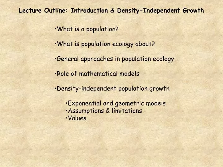
Lecture Outline: Introduction & Density-Independent Growth. What is a population? What is population ecology about? General approaches in population ecology Role of mathematical models Density-independent population growth Exponential and geometric models Assumptions & limitations Values.

E N D
Lecture Outline: Introduction & Density-Independent Growth • What is a population? • What is population ecology about? • General approaches in population ecology • Role of mathematical models • Density-independent population growth • Exponential and geometric models • Assumptions & limitations • Values
What is a population? Gotelli (2001). “A population is a group of individuals, all of the same species, that live in the same place. Although it is difficult to define the physical boundaries of a population, the individuals within the population have the potential to reproduce with one another during the course of their lifetimes.” Akcakaya et al. (1999). “…a collection of individuals that are sufficiently close geographically that they can find each other and reproduce… Thus, it rests on the biological species concept” “In practice, a population is any collection of individuals of the same species distributed more or less contiguously.” Begon et al. (1996).“A group of individuals of one species in an area, though the size and nature of the area is defined, often arbitrarily, for the purposes of the study being undertaken.”
What is population ecology? • The study of how and why the distribution, abundance, and composition of populations change over time and space. • Historical focus on changes in abundance over time • (e.g., population growth models, population cycles). • Current focus includes aspects of spatial structure and dynamics (e.g., dispersal and metapopulations). • Bridge between individual ecology and community ecology, and typically includes two-species interactions (competition, predation, parasitism).
One course objective is to maintain a balance between theory and practical applications of population ecology to wildlife conservation and resource management. “…the places where the imagined world of the mathematician and the real world of the biologist intersect.” Sharon Kingsland (1995) in reference to Population Ecology “Wildlife Population Ecology” Application of principles of population ecology to conserve, restore, manage or control non-domesticated vertebrate species.
Some relevant questions of Wildlife Population Ecology • How does demographic and environmental stochasticity affect our ability to predict the future number of deer based on present number of individuals? • Given data on survival, reproduction, and age structure, what are the chances that a population of an endangered songbird species persists for 100 years? What processes are important to persistence? • How does patch structure, dispersal ability, and environmental correlation affect extinction patterns within a metapopulation? • 4. Do source-sink dynamics affect our ability to evaluate and manage habitat quality for wildlife species? • 5. How does detectability of individuals influence field estimates of population size or survival?
General Approaches to Population Ecology Experimentation Observational Modeling • Observational—includes statistical analysis of time-series data • Modeling—mathematical models of mechanisms • Experimentation—manipulative field studies with controls & replication
Why use models? • Nature is complex so we need to use simplified, abstractions of reality. • Provide a framework for organizing observations and ideas. Alternative is loose collection of isolated facts and case studies. • Generate testable predictions that help us to identify mechanisms responsible for observed patterns. • Expose faulty assumptions. That is, many models are wrong but the reasons for model failure are informative. • Highlight gaps in field data. Help to direct future sampling efforts.
Advantages of mathematical models vs. conceptual models • Require explicit statements of rules and variables, which results in more precise hypotheses. • Equations can unveil emergent properties that are difficult to predict using only non-mathematical reasoning. Dangers of mathematical models in ecology • We build models that are too complex. Models contain many variables that can never be measured in the field and solutions become complex. • We forget that a model is an abstract representation of nature • and that nature might not follow its rules.
Experimentation Observational Modeling • Historically, mathematical models and modelers were viewed with skepticism by many traditional field ecologists (Kingsland 1995). • Many of the modelers were not ecologists, or even biologists (e.g., human demographers, theoretical physicists). Relevance of the models to practical questions was not initially obvious. • In contrast, other ecologists welcomed mathematical approach and hoped it would help to solidify ecology as a hard science • (aka ‘Physics Envy’). • Today, most ecologists agree that studies in population ecology ideally should integrate different approaches (strengths & weaknesses).
Peter Turchin—”Krebs argues that progress inelucidating mechanisms of population regulation can be achieved only by careful experimentation. I strongly disagree with this philosophical stance. …In contrast to Krebs, who argues that we should start with experiments, I propose that we should end with them. The experimental approach is most powerful during the later stages of an investigation into dynamics of any particular population…” But tension among ecologists continues… Charles Krebs-”Avoid mathematical models. They are more seductive than useful at this stage of the subject. If you are addicted to models, at least do not believe them until all of the assumptions can be tested and their predictions verified. There is no such thing in population dynamics as a ‘reasonable assumption’ without data.”
Mathematical modeling Generate predictions to compare to time-series Alternative hypotheses Specific models Experimentation Test predictions supported by the integrated modeling & time series-analysis Turchin’s Approach Time-series analysis • Initial stages of investigation • Quantitative description of patterns of population fluctuations • Potential to reduce number of viable alternatives
Density-independent Population Growth • Simplest model of population growth • Population processes are not affected by current density of population. • Constant fraction is added to population each time step. MULTIPLICATIVE PROCESS • Deterministic models (vs. stochastic models) • Parameters are constant & do not vary unpredictably over time • No uncertainty—given starting conditions, models always produce the same predictions
Discrete vs. Continuous Growth Models • Discrete • Species with non-overlapping generations (some insects) • Species with pulsed reproduction (many wildlife species in seasonal environments) • Time is modeled in discrete steps (often 1 year) • Fits well with annual censuses of wildlife populations • Difference equations are used to model population growth. • Continuous • Species that grow continuously without pulsed births & deaths (humans, some wildlife species in relatively stable environments) • Time is modeled as a continuous, smooth curve • Analytically tractable so you can find solutions using calculus • Differential equations are used to model population growth. For density-independent growth, discrete and continuous models produce qualitatively similar predictions.
Simple models assume a closed population (often not true): Nt+1 = Nt + B – D Nt+1– Nt = B – D ∆N = B - D The “BIDE” Equation Nt+1 = Nt + B + I - D - E B = number of births per time period D = number of deaths per time period I = number of immigrants per time period E = number of emigrants per time period
Geometric Growth (discrete model) • Assume population increases or decreases each year by a constant proportion (z) • If population increases by 25% between years, then z = 0.25. Nt + 1 = Nt + zNt Nt + 1 = (1+ z) Nt Let 1 + z= λ. Lambda is thefinite rate of increase. Nt + 1 = λ Nt **** **** • If λ = 1.25, then population increases 25% per year
Finite rate of increase Nt + 1 = λ Nt Dimensionless ratio, no units λ= Nt + 1/Nt • For example, if population size of coyotes in a study area is 150 this year and size is 200 next year, then lambda equals 1.33 • (200/150). • If λ= 1.33, then population increases 33% per time step (year) λ > 1, exponential increase λ = 1, no change—stationary population λ < 1, exponential decline
Nt + 2 = λλ Nt Nt + 2 = λ2 Nt Nt = λt N0 Where N0 is initial population size. Example: N0 = 100, λ = 1.15, t = 10 years N10 = (1.1510)100 = 405 individuals How do we predict total population size at some particular time? For example, how about for two years in the future? Nt + 2 = λ Nt + 1 Nt + 1 = λ Nt
Note: Akcakaya et al. use big ‘R’ instead of λ for the Finite Rate of Increase in discrete models. Nt = Rt N0
dN/dt = B – D = bN – dN = (b – d) N = rN where b and d are per capita birth and death rates. dN/dt = rN where r is theinstantaneous rate of increase The units of r are individuals/(individuals * time) NOTE: r is also called the intrinsic rate of increase. Exponential Growth (continuous model) • Continuous model is equivalent to a discrete difference equation with an infinitely small time step. • We treat time as being continuous so change in population size is described by a differential equation: r > 0, exponential increase r = 0, no change—stationary population r < 0, exponential decline
Example: N0 = 100, r = 0.1398, t = 10 years N10 = 100(e0.1398)10 = 405 individuals How do we predict total population size at some particular time? We integrate the differential equation dN/dt = rN Nt = N0ert where e is ≈ 2.718
Semi-log plot of population size over time is linear if population is growing exponentially. (from Akcakaya et al.) Population sizes of muskox on Nunivak Island
Linear N Semi-log Slope = r (intrinsic rate of increase) ln(N) Time (t) (from Gotelli)
Two predictive equations for population size Continuous: Discrete: Nt = λt N0 Nt = N0ert Hence, λ = er ln(λ) = r
Doubling Time How long will it take a population to double in size? Nt = λt N0 λt =Nt/N0 If Nt/N0 = 2, what is t? λt = 2 t ln(λ) = ln(2) t = ln(2)/r t = ln(2)/ln(λ) (continuous growth)
Assumptions of Exponential Model • Birth and death rates are constant over time • No competition for limiting resources (no density-dependence) • No random changes over time 2. No age or size structure, and no differences in birth and death rates among individuals. 3. Population is closed. No emigration or immigration. 4. No time lags (for continuous model). 5. No genetic structure.
Where might the exponential model apply? • In the lab. • In nature, but typically for relatively short time periods. • Newly established populations, especially with few predators. • Invasive species, pest outbreaks • Populations recovering from catastrophic declines. • Humans (ability to raise ‘carrying capacity’ over time). Wildlife populations do not increase without bound for very long.
What is the value of exponential growth model? Gotelli: Exponential growth model is the cornerstone of population biology. Turchin: Exponential growth is the first law of population dynamics. Exponential law is similar to laws of physics, such as Newton’s law of inertia. All populations have the potentialfor exponential increase.