Download
1 / 23
230 likes | 358 Vues
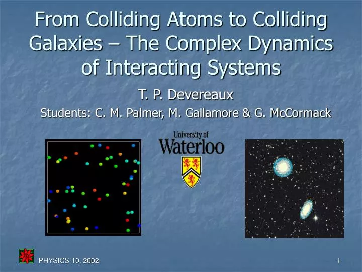
From Colliding Atoms to Colliding Galaxies – The Complex Dynamics of Interacting Systems. T. P. Devereaux Students: C. M. Palmer, M. Gallamore & G. McCormack. Many-Body Physics at Many Length Scales. 10 26 - 10 15 m. 10 2 – 10 -4 m. Universe evolve? Galaxy formation? Cosmic strings?.

E N D
From Colliding Atoms to Colliding Galaxies – The Complex Dynamics of Interacting Systems T. P. Devereaux Students: C. M. Palmer, M. Gallamore & G. McCormack
Many-Body Physics at Many Length Scales 1026 - 1015 m 102 – 10-4 m Universe evolve? Galaxy formation? Cosmic strings? Phases of matter? Neural networks? 10-4 – 10-8 m 1015 - 108 m Cell dynamics? Protein folding? Magnetic vortices in superconductors? Black holes? Star formation? Are orbits stable? 108 - 102 m 10-8 – 10-16 m Global warming? Predict weather? Population biology? Electron transport? Ultra-cold atoms? Forces inside the nucleus?
Start out with 1 particle: F=ma or -iħ∂Ψ/∂t = H Ψ - determines particle’s path. What cannot be explained in terms of non-interacting particles: Collective behavior of many particles (galaxies, proteins, metals, etc.). Phase transitions (e.g. solid-liquid, ferromagnet-paramagnet). Structures and conformations (crystals, polymers, biopolymers, etc.). Instabilities of “particles” or “fields” (1D Luttinger liquid, black holes, cosmic strings). The Many-Body Problem Solving for a particle’s path • Add another particle: • add V(r1-r2) • - path of particle 1 depends on path of particle 2. • Add one more particle… • NOT EXACTLY SOLVABLE! (except in special cases) PROBLEM – How can we approach real systems?
What is Computational Physics?Computation v. Experiment v. Theory in Physics • The goal of computational physics is not to replace theory or experiment, but to enhance our understanding of physical processes. • “Create experiments”. • Visualize physics in action. • Multi-disciplinary. • Cost effective research. • Very accessible.
Different Computational Approaches • Enumeration (e.g. Monte Carlo). • Simulation (molecular dynamics). • Algebraic manipulations (Maple, Mathematica). • Solution of approximate equations (dynamical mean field theory).
Enumeration – Monte Carlo methods Low Temperature High Temperature • Enumerate all the states of a system and determine their energy. • Evolve towards a ground state. Used widely in chemistry, materials physics, and biophysics: Example: Simulated Annealing, Lattice Melting
Simulation: N-Body Tree Codes F=ma for all coupled particles (~106). Widely used in astronomy and condensed matter: Example: Galaxy merger C. Mihos, CWRU `
Approach to Modeling Real Systems • Work on either exact problems or toy models. • Do “experiments” with basic fundamental ideas. • Determine dynamics – macroscopic behavior reproduced? • Determine essential physics ingredient.
Let’s Look at a Specific Problem… 1026 - 1015 m 102 – 10-4 m Universe evolve? Galaxy formation? Cosmic strings? Phases of matter? Neural networks? 10-4 – 10-8 m 1015 - 108 m Cell dynamics? Protein folding? Magnetic vortices in superconductors? Are orbits stable? Star formation? Black holes? • How do structures order? • How are they affected by defects? • How do they respond to external forces? What are magnetic vortices in superconductors? Dynamics of Extended Floppy Objects 108 - 102 m 10-8 – 10-16 m • Lipids, proteins • DNA • Magnetic vortices Predict weather? Global warming? Population biology? Electron transport? Ultra-cold atoms? Forces inside the nucleus?
Real applications of superconductors Mag-lev Transmission lines Biomedical applications • Further applications? • peta-flop supercomputer? • nanoscale devices? • quantum computation?
Vortices in Superconductors • Electrons pair to lower their energy when cooled to superconducting state. • Electrons carry current without resistance and expel magnetic fields. • Electrons swirl in magnetic field –> KE kills superconductivity. • SOLUTION: Rather than kill superconductivity altogether, let magnetic field penetrate in isolated places -> VORTICES (tubes of swirling electrons). EXTENDED FLOPPY OBJECT (you can choose another if you like)!
Visualization of Increasing Applied Magnetic Field B B Now if an external current J is applied… More and more vortices appear as the magnetic field increases… …and the vortices begin to “order” into a lattice. J F Lorentz force causes vortices to move -> EMF produced and we get resistance! NO LONGER A SUPERCONDUCTOR!
Solution: Create defects to pin vortices • Krusin-Elbaum et al (1996). Vortices lower their energy by sitting on defects. • Critical current enhanced over “virgin” material. • Splayed defects better than straight ones. • Optimal splaying angle ~ 4 degrees.
Molecular Dynamics Simulations of Vortices • Vortices = elastic strings under tension. • Vortices repel each other. • Temperature treated as Langevin noise. • Solve equations of motion for each vortex. • Calculate current versus applied Lorentz force, determine critical current.
Animation: Pinning of Vortices • Different types of pinning: • straight • stretched • collective …would be missed if vortices were treated individually.
Pinning Principles (fixed field) At low T, a few pins can stop the whole lattice. At larger T, pieces of lattice shear away. Columnar defects
Pinning principles (fixed temperature) For small fields, pinned vortices may trap others. But “channels” of vortex flow appear at larger fields.
Depinning <-> vortex avalanches • STRATEGY • Use defects to pin, block channel flow. • Take advantage of repulsion. • So we must pin all vortices. • Identified main ingredient – blocking channel flow.
A Wall of Defects? A wall of defects can stop channel flow… …but causes too much damage to sample.
Splaying (tilting) Defects Vortices “stuck” on tilted defects. But vortices have difficulty accommodating to defects for large angles of splay. • Stuck vortices block interstitials. • Channels of flow eliminated.
Reproducing Experiments • Two-stage depinning for columnar defects (squares) – channel flow and onset of bulk flow. Splayed defects (circles) eliminate channels of flow. • Used our simulations to identify main physical ingredient (blocking channel flow) to reproduce experimental behavior.
Ending the story… Computational many body physics is diverse and applicable to many important problems across many fields.
Summary • Many-body problem touches all length scales, many areas of physics. • Computational physics is a powerful and cost-effective tool to complement theory/experiment. • Many roads to follow: • Use N-body tree codes to simulate galaxies and larger scale systems. • Unzipping transitions in DNA; Pathways of protein folding -> Raman (light) scattering. • Onset of avalanches. • Behavior as a qubit (quantum computing).