Download
1 / 33
330 likes | 518 Vues
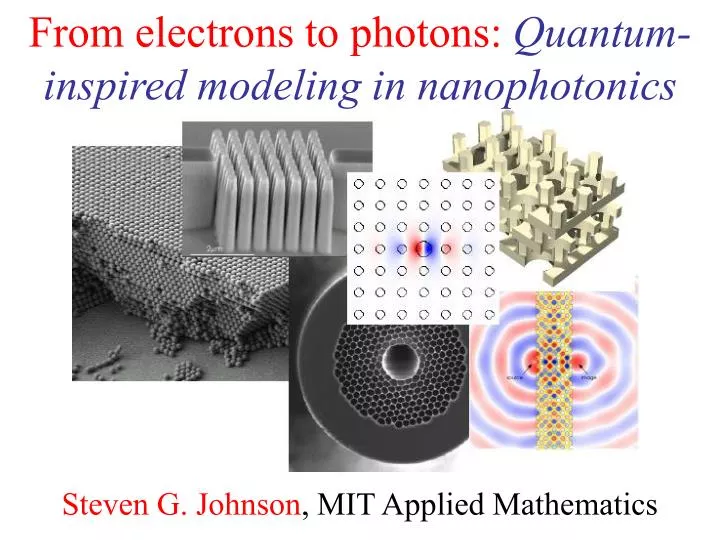
From electrons to photons: Quantum-inspired modeling in nanophotonics. Steven G. Johnson , MIT Applied Mathematics. Nano-photonic media ( l -scale). strange waveguides. & microcavities. [B. Norris, UMN]. [Assefa & Kolodziejski, MIT]. 3d structures . [Mangan, Corning].

E N D
From electrons to photons: Quantum-inspired modeling in nanophotonics Steven G. Johnson, MIT Applied Mathematics
Nano-photonicmedia (l-scale) strange waveguides & microcavities [B. Norris, UMN] [Assefa & Kolodziejski, MIT] 3d structures [Mangan, Corning] synthetic materials optical phenomena hollow-core fibers
1887 1987 Photonic Crystals periodic electromagnetic media can have a band gap: optical “insulators”
dielectric spheres, diamond lattice photon frequency wavevector Electronic and Photonic Crystals atoms in diamond structure Periodic Medium Bloch waves: Band Diagram electron energy wavevector interacting: hard problem non-interacting: easy problem
Electronic & Photonic Modelling Electronic Photonic • strongly interacting —tricky approximations • non-interacting (or weakly), —simple approximations (finite resolution) —any desired accuracy • lengthscale dependent (from Planck’s h) • scale-invariant —e.g. size 10 10 Option 1: Numerical “experiments” — discretize time & space … go Option 2: Map possible states & interactions using symmetries and conservation laws: band diagram
+ constraint eigen-state eigen-operator eigen-value Fun with Math First task: get rid of this mess 0 dielectric function e(x) = n2(x)
Electronic & Photonic Eigenproblems Electronic Photonic simple linear eigenproblem (for linear materials) nonlinear eigenproblem (V depends on e density ||2) —many well-known computational techniques Hermitian = real E & w, … Periodicity = Bloch’s theorem…
A 2d Model System dielectric “atom” e=12 (e.g. Si) square lattice, period a a a E TM H
Periodic Eigenproblems if eigen-operator is periodic, then Bloch-Floquet theorem applies: can choose: planewave periodic “envelope” Corollary 1: k is conserved, i.e.no scattering of Bloch wave Corollary 2: given by finite unit cell, so w are discrete wn(k)
Solving the Maxwell Eigenproblem Finite celldiscrete eigenvalues wn Want to solve for wn(k), & plot vs. “all” k for “all” n, constraint: where: H(x,y) ei(kx – wt) Limit range ofk: irreducibleBrillouin zone 1 Limit degrees of freedom: expand H in finitebasis 2 Efficiently solve eigenproblem: iterative methods 3
ky kx Solving the Maxwell Eigenproblem: 1 Limit range ofk: irreducible Brillouin zone 1 —Bloch’s theorem: solutions are periodic in k M first Brillouin zone = minimum |k| “primitive cell” X G irreducible Brillouin zone: reduced by symmetry Limit degrees of freedom: expand H in finite basis 2 Efficiently solve eigenproblem: iterative methods 3
Solving the Maxwell Eigenproblem: 2a Limit range ofk: irreducible Brillouin zone 1 Limit degrees of freedom: expand H in finite basis (N) 2 solve: finite matrix problem: Efficiently solve eigenproblem: iterative methods 3
Solving the Maxwell Eigenproblem: 2b Limit range ofk: irreducible Brillouin zone 1 Limit degrees of freedom: expand H in finite basis 2 — must satisfy constraint: Planewave (FFT) basis Finite-element basis constraint, boundary conditions: Nédélec elements [ Nédélec, Numerische Math. 35, 315 (1980) ] constraint: nonuniform mesh, more arbitrary boundaries, complex code & mesh, O(N) uniform “grid,” periodic boundaries, simple code, O(N log N) [ figure: Peyrilloux et al., J. Lightwave Tech. 21, 536 (2003) ] Efficiently solve eigenproblem: iterative methods 3
Solving the Maxwell Eigenproblem: 3a Limit range ofk: irreducible Brillouin zone 1 Limit degrees of freedom: expand H in finite basis 2 Efficiently solve eigenproblem: iterative methods 3 Slow way: compute A & B, ask LAPACK for eigenvalues — requires O(N2) storage, O(N3) time Faster way: — start with initial guess eigenvector h0 — iteratively improve — O(Np) storage, ~O(Np2) time for p eigenvectors (psmallest eigenvalues)
Solving the Maxwell Eigenproblem: 3b Limit range ofk: irreducible Brillouin zone 1 Limit degrees of freedom: expand H in finite basis 2 Efficiently solve eigenproblem: iterative methods 3 Many iterative methods: — Arnoldi, Lanczos, Davidson, Jacobi-Davidson, …, Rayleigh-quotient minimization
Solving the Maxwell Eigenproblem: 3c Limit range ofk: irreducible Brillouin zone 1 Limit degrees of freedom: expand H in finite basis 2 Efficiently solve eigenproblem: iterative methods 3 Many iterative methods: — Arnoldi, Lanczos, Davidson, Jacobi-Davidson, …, Rayleigh-quotient minimization for Hermitian matrices, smallest eigenvalue w0minimizes: minimize by preconditioned conjugate-gradient(or…) “variational theorem”
a Band Diagram of 2d Model System(radius 0.2a rods, e=12) frequencyw(2πc/a) = a / l irreducible Brillouin zone G G X M M E gap for n > ~1.75:1 TM X G H
Preconditioned conjugate-gradient: minimize (h + a d) — d is (approximate A-1) [f + (stuff)] The Iteration Scheme is Important (minimizing function of 104–108+ variables!) Steepest-descent: minimize (h + a f) over a … repeat Conjugate-gradient: minimize (h + a d) — d is f+ (stuff): conjugate to previous search dirs Preconditioned steepest descent: minimize (h + a d) — d = (approximate A-1) f ~ Newton’s method
The Iteration Scheme is Important (minimizing function of ~40,000 variables) no preconditioning % error preconditioned conjugate-gradient no conjugate-gradient # iterations
E|| is continuous E is discontinuous (D = eE is continuous) Any single scalare fails: (mean D) ≠ (anye) (mean E) Use a tensore: E|| E The Boundary Conditions are Tricky e?
The e-averaging is Important backwards averaging correct averaging changes order of convergence from ∆x to ∆x2 no averaging % error tensor averaging (similar effects in other E&M numerics & analyses) resolution (pixels/period)
Gap, Schmap? a frequencyw G G X M But, what can we do with the gap?
Intentional “defects” are good microcavities waveguides (“wires”)
(Same computation, with supercell = many primitive cells) Intentional “defects” in 2d
Microcavity Blues For cavities (point defects) frequency-domain has its drawbacks: • Best methods compute lowest-w bands, but Nd supercells have Nd modes below the cavity mode — expensive • Best methods are for Hermitian operators, but losses requires non-Hermitian
Time-Domain Eigensolvers(finite-difference time-domain = FDTD) Simulate Maxwell’s equations on a discrete grid, + absorbing boundaries (leakage loss) • Excite with broad-spectrum dipole ( ) source Dw Response is many sharp peaks, one peak per mode signal processing complexwn [ Mandelshtam, J. Chem. Phys.107, 6756 (1997) ] decay rate in time gives loss
Signal Processing is Tricky signal processing complexwn ? a common approach: least-squares fit of spectrum fit to: FFT Decaying signal (t) Lorentzian peak (w)
There is a better way, which gets complex w to > 10 digits Fits and Uncertainty problem: have to run long enough to completely decay actual signal portion Portion of decaying signal (t) Unresolved Lorentzian peak (w)
There is a better way, which gets complex w for both peaks to > 10 digits Unreliability of Fitting Process Resolving two overlapping peaks is near-impossible 6-parameter nonlinear fit (too many local minima to converge reliably) sum of two peaks w = 1+0.033i w = 1.03+0.025i Sum of two Lorentzian peaks (w)
Idea: pretend y(t) is autocorrelation of a quantum system: time-∆t evolution-operator: say: Quantum-inspired signal processing (NMR spectroscopy):Filter-Diagonalization Method (FDM) [ Mandelshtam, J. Chem. Phys.107, 6756 (1997) ] Given time series yn, write: …find complex amplitudes ak & frequencies wk by a simple linear-algebra problem!
…expand U in basis of |(n∆t)>: Umn given by yn’s — just diagonalize known matrix! Filter-Diagonalization Method (FDM) [ Mandelshtam, J. Chem. Phys.107, 6756 (1997) ] We want to diagonalize U: eigenvalues of U are eiw∆t
Filter-Diagonalization Summary [ Mandelshtam, J. Chem. Phys.107, 6756 (1997) ] Umn given by yn’s — just diagonalize known matrix! A few omitted steps: —Generalized eigenvalue problem (basis not orthogonal) —Filter yn’s (Fourier transform): small bandwidth = smaller matrix (less singular) • resolves many peaks at once • # peaks not knowna priori • resolve overlapping peaks • resolution >> Fourier uncertainty
Do try this at home Bloch-mode eigensolver: http://ab-initio.mit.edu/mpb/ Filter-diagonalization: http://ab-initio.mit.edu/harminv/ Photonic-crystal tutorials(+ THIS TALK): http://ab-initio.mit.edu/ /photons/tutorial/

![Data Modeling [Comparison of data modeling techniques ]](https://cdn0.slideserve.com/205866/data-modeling-comparison-of-data-modeling-techniques-dt.jpg)