Download
1 / 47
560 likes | 1.53k Vues
2. For next time:Read: ? 8-11 to 8-13, 9-1 to 9-2.HW12 due Wednesday, November 19, 2003Outline:Rankine steam power cycleCycle analysisExample problemImportant points:Know what assumptions you can make about the points along the cycle pathKnow how to analyze a pumpKnow how all the isentr

E N D
1. 1 Lec 23: Brayton cycle regeneration, Rankine cycle
2. 2 For next time:
Read: � 8-11 to 8-13, 9-1 to 9-2.
HW12 due Wednesday, November 19, 2003
Outline:
Rankine steam power cycle
Cycle analysis
Example problem
Important points:
Know what assumptions you can make about the points along the cycle path
Know how to analyze a pump
Know how all the isentropic efficiencies are defined
3. 3 Improved Brayton Cycle: Add a Heat Exchanger (Regenerator)
4. 4 Ts Diagram for Brayton Cycle with Regeneration
5. 5 Analysis with regeneration
6. 6 Analysis with regeneration
7. 7 Regenerator in cycle
8. 8 Regenerator Effectiveness
9. 9 Efficiency with regeneration
10. 10
11. 11
12. 12
13. 13
14. 14
15. 15 TEAMPLAY
16. 16 Vapor Power Cycles The Carnot cycle is still important as a standard of comparison.
However, just as for gas power cycles, it cannot be practically achieved in useful, economical systems.
17. 17 We�ll simplify the power plant
18. 18 Ideal power plant cycle is called the Rankine Cycle 1-2 reversible adiabatic (isentropic) compression in the pump
2-3 constant pressure heat addition in the boiler.
3-4 reversible adiabatic (isentropic) expansion through turbine
4-1 constant pressure heat rejection in the condenser
19. 19 Rankine cycle power plant The steady-state first law applied to open systems will be used to analyze the four major components of a power plant
Pump
Boiler (heat exchanger)
Turbine
Condenser (heat-exchanger)
The second law will be needed to evaluate turbine performance
20. 20 Vapor-cycle power plants
21. 21 What are the main parameters we want to describe the cycle?
22. 22 Main parameters�.
23. 23 General comments about analysis Typical assumptions�
Steady flow in all components
Steady state in all components
Usually ignore kinetic and potential energy changes in all components
Pressure losses are considered negligible in boiler and condenser
Power components are isentropic for ideal cycle
24. 24 Start our analysis with the pump
25. 25 Pump Analysis
26. 26 Boiler is the next component.
27. 27 Proceeding to the Turbine
28. 28 Last component is the Condenser
29. 29 More condenser...
30. 30 Ideal Rankine Cycle The pump work, because it is reversible and adiabatic, is given by
31. 31 Ideal Rankine Cycle on a p-v diagram
32. 32 Efficiency
33. 33 Example Problem
34. 34 Start an analysis:
35. 35 Draw diagram of cycle
36. 36 Some comments about working cycle problems Get the BIG picture first - where�s the work, where�s the heat transfer, etc.
Tables can useful - they help you put all the data you will need in one place.
You will need to know how to look up properties in the tables!
37. 37 Put together property data
38. 38 Property data h1=191.83 kJ/kg is a table look-up, as is h3=3582.3 kJ/kg.
39. 39 Let start with pump work
40. 40 More calculations...
41. 41 Calculate heat input and turbine work..
42. 42 Property data Because s3= s4, we can determine that x4=0.803 and thus h4=2114.9 kJ/kg
43. 43 Turbine work
44. 44
45. 45 Overall thermal efficiency
46. 46 Some general characteristics of the Rankine cycle Low condensing pressure (below atmospheric pressure)
High vapor temperature entering the turbine (600 to 1000?C)
Small backwork ratio (bwr)
47. 47 TEAMPLAY


![Tricarboxylic acid cycle (TCA Cycle) [Kreb’s cycle] [Citric acid cycle]](https://cdn2.slideserve.com/5062555/tricarboxylic-acid-cycle-tca-cycle-kreb-s-cycle-citric-acid-cycle-dt.jpg)