Download
1 / 10
100 likes | 448 Vues
Example: Southern redback salamander, Plethodon serratus. Terrestrial salamander in southern Appalachians Abundance is difficult to estimate Highly variable counts from natural cover or coverboard sampling Likely that p < 1. 50m. 10m. 10m. 10m. “Site” Design. Natural Cover Transect.

E N D
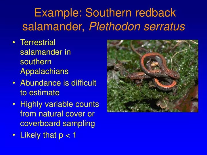
Example: Southern redback salamander, Plethodon serratus • Terrestrial salamander in southern Appalachians • Abundance is difficult to estimate • Highly variable counts from natural cover or coverboard sampling • Likely that p < 1
50m 10m 10m 10m “Site” Design Natural Cover Transect 3m Cover Boards Sampling Details 39 “Sites” sampled 4 Years (1998-2001) Sampled 5 times/year
Plethodon serratus Occupancy : Hypotheses • Expect probability of occupancy influenced by previous disturbance history, (dist). • Expect temporal variation in occupancy and colonization probabilities due to variations in annual rainfall (declined 1999-2001 for April-June months). • Expect temporal variation in detection probabilities due to yearly rainfall variations, p (year •), or consistent yearly patterns of seasonal availability, p (• t).
Plethodon serratus Occupancy : Modeling • Model parameterization: (t, t ) • Candidate Models include combinations of: • Occupancy (3 levels): - y(•) : Occupancy constant - y(dist): Occupancy varies by disturbance history - y(year): Occupancy varies by year • Colonization (2 levels): • γ(•): Colonization constant • γ(year): Colonization varies by year • Detection (3 levels): • p(•): Detection constant • p (year •): Detection varies due to yearly rainfall • p(• t): Detection varies due to seasonal availability within the sampling season
Compare Models with p(• t) AIC ∆ AIC K Ψ 1998 Ψ 1999 Ψ 2000 Ψ 2001 p(1) p(5) Ψ(dist)γ(•)p(• t) 752.5 0.00 8 0.94 (0.42) 0.94 (0.42) 0.94 (0.42) 0.94 (0.42) 0.85 0.23 Ψ(•)γ(•)p(• t) 766.2 13.7 7 0.79 0.79 0.79 0.79 0.85 0.23 Ψ(•)γ(year)p(• t) 769.4 16.9 9 0.78 0.78 0.78 0.78 0.85 0.23 Ψ(year)γ(•)p(• t) 771.6 19.4 8 0.82 0.81 0.79 0.76 0.86 0.23 Naïve Estimates 0.58 0.82 0.82 0.74 p(• t) Model Results: Occupancy & Detection K = number of parameters. For models with Ψ(dist),the first occupancy estimate is for undisturbed sites, followed by disturbed site estimate in parentheses. Only detection probabilities for first & last sample reported.
Compare Models withp(• t) w ∆ AIC K γ 1998 γ 1999 γ 2000 Ψ(dist)γ(•)p(• t) 0.99 0.00 8 0.21 0.21 0.21 Ψ(•)γ(•)p(• t) 0.01 13.7 7 0.22 0.22 0.22 Ψ(•)γ(year)p(• t) 0.00 16.9 9 0.32 0.25 0.14 Ψ(year)γ(•)p(• t) 0.00 19.4 8 0.17 0.17 0.17 Naïve Estimates 0.28 0.05 0.00 p(• t) Model Results: Colonization K = number of parameters. w = Akaike weight, evidence (probability) the given model is the ‘best’
p(year •) Model Results: Occupancy & Detection K = number of parameters. For models with Ψ(dist),the first occupancy estimate is for undisturbed sites, followed by disturbed site estimate in parentheses.
p(year •) Model Results: Colonization K = number of parameters. w = Akaike weight, evidence (probability) the given model is the ‘best’
p(• •) Model Results: Occupancy & Detection K = number of parameters. For models with Ψ(dist),the first occupancy estimate is for undisturbed sites, followed by disturbed site estimate in parentheses.
p(• •) Model Results: Colonization K = number of parameters. w = Akaike weight, evidence (probability) the given model is the ‘best’