Download
1 / 70
710 likes | 1.07k Vues
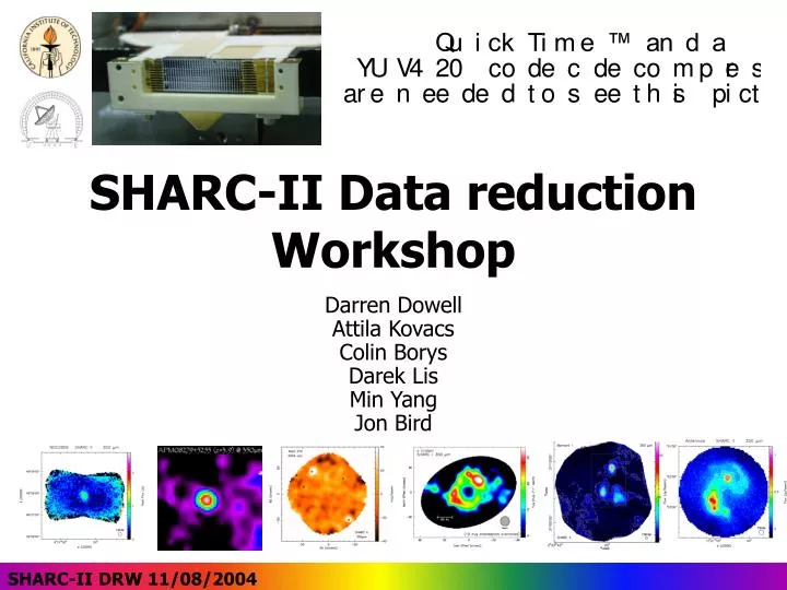
SHARC-II Data reduction Workshop. Darren Dowell Attila Kovacs Colin Borys Darek Lis Min Yang Jon Bird. SHARC-II DRW 11/08/2004. Outline. GOALS Caltech success stories Software Requirements and Installation Overview of available software Installation overview Scripting with CRUSH

E N D
SHARC-II Data reduction Workshop Darren Dowell Attila Kovacs Colin Borys Darek Lis Min Yang Jon Bird SHARC-II DRW 11/08/2004
Outline • GOALS • Caltech success stories • Software Requirements and Installation • Overview of available software • Installation overview • Scripting with CRUSH • CRUSH vs SHARCSOLVE • General SHARC-II Calibration • Opacity (tau) estimation • Calibrators at 350 micron • Stability of calibration • Calibrating your data • Aperture Photometry • PSF Photometry • Example • Map tweaks and presentation • Pointing, Calibration, Coadding, Cropping, and Mosaicing • Making publishable images with IDL • Chopped data • Lessons learned • Tips for taking better data • Miscellaneous notes SHARC-II DRW 11/08/2004
Goals 1. Transfer expertise from Caltech to other users Why? To promote publication of SHARC-II data Transfer expertise from other users to Caltech Why? Users tend to be familiar with the issues involved. 3. Learn about difficulties users have with instrument/data Why? To improve the system. 4. Improve data acquisition techniques Why? Improve efficiency of SHARC-II observations SHARC-II DRW 11/08/2004
Caltech Success Stories The next few slides present results from observations conducted by members of the Caltech SHARC-II group. They span a variety of flux levels and redshifts, and are meant to illustrate the full range of SHARC-II’s abilities. SHARC-II DRW 11/08/2004
SLUGS (z<0.05) • Dunne et al. have characterized the SED of 106 IRAS selected galaxies at 850m • Of those, only 17 were detected by SCUBA at 450 m, and it was noted that the data supported a 2-component SED fit. • SHARC-II has detected roughly 60/65 targeted so far. • They are so easy to detect that they now are done as poor-weather backup. • 0.5h @ 225~0.06 • 1.0h @ 225~0.08 • 0.5 Jy< S350 < 3 Jy • crush -faint -compact SHARC-II DRW 11/08/2004
Spitzer HLIRG (z~1.5) • In follow-up observations of Spitzer selected objects, we discovered an object with an apparent luminosity above 1013.5 L. • It has an SED similar to Arp220, but at at a redshift of 1.5. • This object has sparked interest in “Silicate Dropouts” as a way to select high-z starbursts. • 0.5h @ 225~0.06 • S350 = 226 ± 45 mJy • CHOPPED observing • sharcsolve reduction SHARC-II DRW 11/08/2004
Stanford sample (0.1<z<1.0) • The Stanford sample was compiled from cross-correlation of the faint-IRAS catalog and the FIRST 21cm radio catalog • The sources are ULIRG’s lying within redshift range of 0.1 and 1; NIR morphologies of these objects reveal they tend to be interacting systems • FIR/submillimeter fluxes were obtained for the first time on these targets, so were SED fits in the FIR 2h @ 225~0.05 S350 = 44.1 mJy Td = 40.9 K , = 1.5 SHARC-II DRW 11/08/2004
Fomalhaut Debris Disk • 3.0h @ 225~0.039 • SWEEP (Lissajous) • crush -deep reduction • Peak fluxes: 150 mJy/beam • Integrated flux: 1.2 Jy • Consistent with thin, uniform dust ring K. Marsh et al. (2004-5) SHARC-II DRW 11/08/2004
Orion Johnstone & Bally (1999) Houde et al. (2004) rms: 0.3 Jy/beam rms: 0.3 Jy/beam rms: 1 Jy/beam rms: 0.3 Jy/beam 4 hr. 1.2 mm PWV 18 hr. 1.0 mm PWV mosaic of BOX scans SHARC-II DRW 11/08/2004
Low-z Interacting Galaxy Survey • Selected by IRAS 100 mm flux and proximity using criterion of Surace (2004). • Perhaps analogues to z>1 ULIRGs. • Lissajous scans in typically t225×airmass = 0.05-0.10. • Observations of 14/42 sources complete, to be reported by J. Bird and D. Dowell. 5×10¹⁰ Lsolar SHARC-II DRW 11/08/2004
CHOP in azimuth 39″/1.39 Hz plus slow SWEEP parallactic angle rotation of 77° washes out negative beams in sharcsolve reduction 8.6 hrs, median tau225 = 0.044 rms = 10 mJy/beam in middle 2 sources are 80 mJy each Definite and probable SCUBA 850 mm sources marked with stars Chopped High-z survey SHARC-II DRW 11/08/2004
High-z SCUBA sources • 3-4h @ 225<0.06 • 350 = 5 mJy LE2 LE31 LE12 LE21 SHARC-II DRW 11/08/2004
Software and Requirements CRUSH is Java based and written and maintained by A. Kovacs Available on web page Has been successfully used on: • Windows • Mac OSX • Linux • Solaris SHARCSOLVE is C based and written by D. Dowell (phasing out?) Available only by special request Has been successfully used on: • Mac OSX • Linux • Solaris Ancillary software written by C. Borys. Available on web page Has been successfully used on: • Mac OSX • Linux • GCC compatible, so in principle could be compiled on other platforms. (C. Borys) Minimum requirements to run all the software are: Java 1.4.1 (for CRUSH) gcc version 3.2.3 cfitsio libraries (http://heasarc.gsfc.nasa.gov/docs/software/fitsio/fitsio.html) Other nice software include: IDL or graphic (for plotting) DS9, GAIA (starlink) for displaying fits files. SHARC-II DRW 11/08/2004
Overview of Ancillary software : 1 header_update : alters header keywords in maps generated by CRUSH. boxscan : helps calculate BOX_SCAN parameters for SHARC-II observations. • See SHARC-II web page for more details sharccal : applies a calibration to a reduced sharc2 signal and noise map sharccal [-c scalefactor] [-o offset] [-v] [-u units] raw.fits calibrated.fits If no options, it will use the builtin calibration factor (V2JY in fits file) Output signal = scalefactor*(raw map + offset) FITS keywords added or modified: NAME value comment ---- ----------- ------------------ V2JY scalefactor calibration factor CALAP T calibration applied? OFFAP T|F offset applied? OFFSET value offset value (only if OFFAP=T) BUNIT unit Units of output image sharcgap : tests a raw sharc2 data file for timing gaps sharcgap startidx stopidx Needs to be run from the directory in which data is stored. It checks consecutive data points to see if they are spaced by more than 1% of the expected time. Expected time is 36ms, but is calculated explicitly from the first HDU. sharcsmooth : Performs a PSF fit to a reduced SHARC2 map. This will be described later in the calibration section. SHARC-II DRW 11/08/2004
Overview of Ancillary software : 2 sharclog : Gets basic information from a SHARC-II raw data file sharclog startidx stopidx Needs to be run from the directory in which data is stored. It scans the header of each file to provide a summary of the data (similar to Darren’s) sharcstat : computes basic statistics on a reduced SHARC2 map sharcstat file.fits > sharcstat zw247_2.fits NX NY N s_mean s_stddev rms_mean rms_stddev 118 76 5049 0.00049829 0.14564 0.023233 0.0072745 N = number of pixels with data in them (checks for NaN). S_ corresponds to mean and standard deviation of the SIGNAL map Rms_ corresponds to mean and standard deviation of the NOISE map. sharctau : uses Jon Bird's tau fits to estimate tau for a given SHARC2 file. You also need the taufit files sharctau [-v] datafile taufile Can be run from anywhere > sharctau -v /home/bigdisk1/sharc2-012900.fits /scr/borys/sharc/tau225_sep2003.fit # DD/MM/YYYY HH:MM UT/24 TAU225 FITTAU # 30/09/2003 12:06 0.50 0.051 0.068 > sharctau /home/bigdisk1/sharc2-012900.fits /scr/borys/sharc/tau225_sep2003.fit 0.068 Note: tau225 is read from file. Fittau is at the frequency appropriate to the input taufile. SHARC-II DRW 11/08/2004
Installation • Create a convenient place for the CRUSH installation. • Use logical links to point to the most recent version. • CRUSH can ONLY be run from the directory in which it is installed. istari (7:45am) [/scr/borys/sharc/attila] >ls -la lrwxrwxrwx 1 borys cittgp 10 Nov 5 08:21 crush -> crush-1.34 drwxr-xr-x 3 borys cittgp 4096 Oct 3 07:16 crush-1.33 drwxr-xr-x 3 borys cittgp 4096 Sep 22 09:39 crush-1.33b2 drwxr-xr-x 3 borys cittgp 4096 Oct 6 15:48 crush-1.34 drwxr-xr-x 2 borys cittgp 4096 Aug 31 23:13 data drwxr-xr-x 3 borys cittgp 4096 Oct 28 00:35 devel drwxr-xr-x 2 borys cittgp 4096 Feb 13 2004 MaiTau • Create a convenient place for the ancillary software. • Add the directory to your PATH variable • These programs can be run from anywhere. istari (7:48am) [/scr/borys/sharc/code/bin] >ls -la -rwxr-xr-x 1 borys cittgp 6793 Aug 27 14:31 boxscan -rwxr-xr-x 1 borys cittgp 16548 Aug 27 14:10 sharccal -rwxr-xr-x 1 borys cittgp 784529 Mar 26 2003 sharcextract -rwxr-xr-x 1 borys cittgp 766548 Aug 27 14:31 sharcgap -rwxr-xr-x 1 borys cittgp 770786 Aug 27 14:31 sharclog -rwxr-xr-x 1 borys cittgp 770704 Aug 27 14:32 sharcsmooth -rwxr-xr-x 1 borys cittgp 16164 Aug 27 14:13 sharcstat -rwxr-xr-x 1 borys cittgp 766589 Aug 27 14:32 sharctau SHARC-II DRW 11/08/2004
Scripting The necessity of running CRUSH from its install directory makes file management slightly tricky. Ways of manipulating output name include: • 1) -outpath= OR REDUCED_MAP_PATH in crush.cfg • This will change the path in which the file is saved, but not alter the name itself. i.e. it will keep the form OBJNAME.SCAN1.SCAN2…SCANN.fits • This filenaming structure is sometimes inconvenient (e.g. GAIA) • 2) -name=/path/to/mapdir/map.fits • This will alter the name to one of your choosing. You can include a path here as well. If used, outpath is ignored. RECOMMENDATION: use scripts and the -name= option #!/bin/csh cd /scr/borys/sharc/attila/crush echo “PROCESSING ic5634” ./crush -faint -compact -name=ic5634_1.fits 14176 14177 >! ic5634_1.log ./crush -faint -compact -name=ic5634_2.fits 14182-14185 >! ic5634_2.log ./coadd -out=ic5634.fits ic5634_1.fits ic5634_2.fits >! ic5634.log sharcsmooth ic5634.fits ic5634_smooth.fits mv -f ic5634* /scr/borys/sharc/projects/slugs/CRUSH/maps/. Note the 2 different ways of specifying scans to analyze SHARC-II DRW 11/08/2004
CRUSH At this point in the workshop, Attila gave a presentation on CRUSH. Download that separately and review it before proceeding. SHARC-II DRW 11/08/2004
Important Differences between CRUSH and SHARCSOLVE • Pointing • Different treatment of the case that the IRC Reference Pixel is not the middle of the array (16.5, 6.5) • Calibration • CRUSH and sharcsolve use completely different units, so cannot mix. • CRUSH corrects for dependence of detector gain on detector loading, so resulting tau relations should look “normal” to SCUBA and SHARC users: (SHARC II, 350 m) ≈ 25(225 – 0.01) • sharcsolve does NOT correct for gain change, so tau scaling looks “too big”: (SHARC II, 350 m) ≈ 32(225 – 0.01) • Chopped reduction • sharcsolve differences with respect to chopper as first step. • CRUSH treats secondary chopping as merely another pointing offset. • Relative advantages of two approaches under study. SHARC-II DRW 11/08/2004
Tau and Calibration • Calibration at short sub-mm wavelengths is challenging, but necessary. • In the next few slides, we present our procedure for estimating the atmospheric opacity, and then discuss the overall calibration uncertainty for SHARC-II • Then we provide a more detailed example of how to obtain the calibrated flux for a specific observation. SHARC-II DRW 11/08/2004
SHARC-II Calibrators • Availability of calibration sources has always been a problem in sub-mm observations, particularly at shorter wavelengths (can’t use BLAZARS, etc) • We use primary calibrators (Mars, Uranus, and Neptune) to bootstrap the calibration of the secondary systems. • For stationary objects, we can use repeated observations to derive averages. • For solar system objects, we need to consider the changes in distance and solid angle over time. • TB = T1AUr(-1/2) • S() = B(TB) • T1AU is derived by evaluating TB given all the other parameters (r is the heliocentric distance in AU, is the solid angle as seen from Earth, and B is the Planck function evaluated at the appropriate frequency (typically 350 micron). These values are provided by the JPL Horizons System: http://ssd.jpl.nasa.gov/cgi-bin/eph • We have used these relations to extrapolate the fluxes for all days between 2002 and 2010. • These calibrations are available for download for the SHARC-II web page SHARC-II DRW 11/08/2004
Tau Fits • Tau Dippers are noisy by nature (single measurement every ~10 min). • Fits for both the 225Ghz and 350 micron data exist for every SHARCII night to date. • Least square polynomial fits over a large range of each night (almost always covering the entire observing time). • Images of these fits are located on the SHARCII website (www.submm.caltech.edu/~sharc). • When reducing your data, observers should look at these tau fits as a FIRST step, so that they may determine the best fit to use and what was happening in the atmosphere at the time of observation. SHARC-II DRW 11/08/2004
Tau Fits Typical 350 micron fit. Residuals are located on bottom of plot. Typical fit ranges from 2 to 20 hours UT. Notice that the X axis is in fraction of a day. SHARC-II DRW 11/08/2004
Keep an eye on the 225GHz and 350 micron fits…they CAN differ Fits from both tippers on the same night. SHARC-II DRW 11/08/2004
CRUSH and Tau • CRUSH uses the MaiTau server to obtain the fitted tau. • Parses through fit table (see below). Available online in conjunction with the tau fits. • CRUSH’s output will inform you if a fit for your file was found and what value was retrieved. “Got Mai-Tau! tau(350um) = X” By default, MaiTau looks at the 350 micron fits. Use “-taufit=” option to choose which fit, or not to use a fit at all. SHARC-II DRW 11/08/2004
Mai Tau success story on Mon R2 Below are maps made from individual scans of MonR2 (provided by D. Benford). The raw tau recorded in the file was used. Problem: Much variability.
Mai Tau success story on Mon R2 Below are maps made from individual scans of MonR2 (provided by D. Benford). Opacity this time was provided by MaiTau. MaiTau helps!
SHARC-II and Calibration Want to determine how stable that conversion factor, and thus calibration, is over time. • Perform aperture photometry on calibrators with “known” fluxes. • “Known” fluxes are obtained from HORIZONS. • CRUSH’s default output is in Volts- constant Volts to Janskys applied (crush.cfg). • By comparing known flux with CRUSH reported flux, we obtain a conversion factor. SHARC-II DRW 11/08/2004
Calibration Stability Plot shows conversion factor of calibrators taken during the August-September 2004 run. Conversion factor is consistent to within: 21.3% for all 18.8% for Neptune 19.2% for Uranus SHARC-II DRW 11/08/2004
Calibration Stability Calibration is consistent over a wide range of elevations. You do not need to take calibration scans at the same elevation as your science. SHARC-II DRW 11/08/2004
Calibration/Tau summary • Tau fits: Important for understanding what is happening to the atmosphere during observation. • Always look at the tau fits as a first step towards calibration and reduction. • CRUSH calibration is now consistent to within 20% and improving. • Calibration is consistent over the range of telescope positions. • In the next few slides, we concentrate on object specific calibrations. SHARC-II DRW 11/08/2004
Calibration : PSF PSF Photometryis the most often used technique for point source extraction in SCUBA maps (particularly high-z projects). It is mathematically equivalent to “convolving with the beam”, except it also takes into account the pixel-to-pixel noise differences. The procedure is very straightforward. Start at a given pixel (i,j), and calculate the following statistic: S and N are the signal and noise maps respectively. This is simply a LLS fit, and it is easy to derive the best fit value and error for the PSF’s amplitude, A. This can be extended to include an offset parameter as well. The ancillary program sharcsmooth performs this function. It assumes a purely Gaussian, with a default (but user settable) FWHM of 9”. (see imagetool as well) The map answers the following statistical question: what is the best fit amplitude to a Gaussian centered at a given pixel? There are consequences to this assumption. i.e., for pixels near the peak of a source, the assumption that that given pixel is the center of a source is wrong. Source extractionwith a “smoothed” map is done by setting a SNR threshold to search for sources in the field. SHARC-II DRW 11/08/2004
Calibration : Aperture Aperture Photometryis another popular choice, most often used on sources that are readily visible in the map, or if some other astrometric marker is available on which the aperture can be centered. There are 3 circular radii to choose. In order of increasing value they are: source, inner sky, and outer sky. The annulus defined by the last two radii are used to estimate the mean sky level AND the scatter of pixels. The central aperture is used to sum up the flux contained within it (after correction for the mean sky offset). The error on the flux estimate is related to the RMS of the pixels in the sky annulus, and the number of pixels in both the aperture and annulus. Aperture radii usually chosen via “curve of groth”, annuli choosen to minimize noise while still providing a good estimate of sky background and RMS. Given that the pixel to pixel errors are dominated by residuals in the sky estimation and not shot and photon noise as they are in optical CCD work, the equations are simpler. Note that CRUSH and SHARCSOLVE do provide a “noise” map, but I have always found that the RMS scatter in the “signal” pixels is higher than what the weight map implies. Thus I assume a uniform weight per map pixel, and calculate this weight via the RMS of the signal map. (implications for PSF fitting…) It is not yet clear to me that sky estimation is necessary. CRUSH and SHARCSOLVE do a pretty good job of returning “zero” for a map mean when we look at blank sky. However, experience has also shown that well detected sources sometimes have a negative “bowl” around them. SHARC-II DRW 11/08/2004
Calibration : Aperture Important caveat: This procedure assumes that the pixels are uncorrelated. This is NOT the default procedure for CRUSH, and one has to use -convolve=-1 to force this. Otherwise, the RMS calculation will be lower then it is supposed to be (you’ve essentially smoothed the map). If you do not use the convolve flag, the RMS should be increased by a factor of sqrt(N), where N = the number of pixels that fall within the area of the convolving function. By default, we use an 8” beam, with noise calculated for ~4.8” pixels, which therefore requires a sqrt(1.33)*(8/1.4) = 6.6 increase in RMS (and consequently the total error budget). SHARC-II DRW 11/08/2004
Aperture vs. PSF So which should you use, and what are some caveats? POINT SOURCES If the PSF is varying (ie, DSOS not functioning or not turned on), APERTURE is probably the safer choice. If CHOPPING, care must be taken to keep the annulus away from the offbeams (a concern for SHARCSOLVE, not CRUSH), hence PSF might be a good choice. What do I use? Aperture, almost exclusively, but use the PSF smoothed map for presentation. EXTENDED SOURCES PSF, since it essentially gives you Flux/beam. CAVEATS In deep integrations, there are some issues related to correlated sky signal still in the map. (more from Attila) SHARC-II DRW 11/08/2004
Calibrating your data • The principles involved with calibrating SHARC-II data are applicable to all data from other sub-mm telescopes. • Ingredients • Good estimates of the atmospheric opacity for all science and calibration observations • A decent collection of calibrators (different objects, airmasses, etc.) • A CHOICE IN HOW YOU WILL EXTRACT FLUXES FROM YOUR DATA. What is done to the science map must also be done to the calibration. • EXAMPLE: Reduction of a local IRAS galaxy: MRK 331 • Scans 9125-9127, taken on Jan 15, 2003, at UT 04:54 • PSF photometry to be used SHARC-II DRW 11/08/2004
Calibration Example 1 Using sharclog, (or by some other log or by looking at the header), I find the UT time and date the data were taken, and then go to the SHARC-II web page to get the tau-fit plot for that night. The data were taken at UT 04:30 (~0.20 fractional day). Fits look OK, so I will not override MaiTau. Next I run CRUSH to make the map SHARC-II DRW 11/08/2004
Calibration Example 2 > ./crush -faint -compact -convolve=-1 -name=mrk331.fits 9125-9127 >! mrk331.log > sharcsmooth mrk331.fits mrk331_smooth.fits > cat mrk331.log • crush -- Comprehensive Reduction Utility for SHARC2 • Author: Attila Kovacs <attila@submm.caltech.edu> • Version: 1.34-1 • Scan 1: Reading /home/bigdisk1/sharc2/sharc2-009125.fits... • Got Mai-Tau! tau(350um) = 1.3088 • 83 HDUs, 16439 x 36ms frames -> 9.9 minutes total. • Filtering 13.4Hz on noisy pixels. • DownSampling -> 5479 frames • [MRK331] observed at 2003-01-15T04:54:01.949 • RA = 23:48:54.0 DEC = 20:18:29.0 (1950.0) • = 23:51:26.7 = 20:35:10.1 (2000.0) • AZ = 277:44:54.5 EL = 57:01:57.9 • RAO = 0.0 DECO= 0.0 AZO = 0.0 ZAO =-0.0 • FAZO=-104.0 FZAO=-30.0 Rotator = 60.0 RotZero = 60.0 • Pointing Center = 16.5,6.5 Rotation Center = 18.5,8.6 • Parallactic Angle = 85.0 tau225 = 0.053 tau = 1.835 • Plate Scale = 4.93"x4.77" SHARC-II DRW 11/08/2004
Calibration Example 3 • Now I check the logs for that date to see which calibrators were done. • In this particular case, I will only pick the one closest to the science observation, but you should reduce ALL of them and ensure that they seem reasonable. > ./crush -compact -convolve=-1 -name=oh231.fits 9140 >! oh231.log > sharcsmooth oh231.fits oh231_smooth.fits • The sharcsmooth program does a PSF fit to each pixel, so to calibrate, I load the image in GAIA (or DS9) and determine the brightness of the peak. In this case it is 3.378 units. • The true flux of OH231.8 is 19.4±1.9 Jy (10% calibration uncertainty). • Hence the scale factor is: 19.4/3.4 = 5.7 • Now we need to scale our image: > sharccal -c 5.7 -u Jy mrk331_smooth.fits mrk_cal.fits • Finally I open up GAIA, and look at mrk_cal.fits. By looking at the Signal and RMS maps, I see that the brightest pixel is: • 1.80 ± 0.02 Jy • In this case the calibration uncertainty dominates the error budget, so I simply quote 1.8 ± 0.2 Jy. SHARC-II DRW 11/08/2004
Map Tweaks Making the maps is the first step, and you may need/want to perform some of the tweaks presented on the following slides. SHARC-II DRW 11/08/2004
Tweaks-Pointing Correction • Two options for pointing correction: • Apply knowledge of improved telescope pointing model at time of running CRUSH: • crush -FAZO=-120.0 -FZAO=40.0 … • See “MEMO: SHARC II Pointing at Nasmyth Focus Using CRUSH (Dowell, Nov. 2004)” on web page/Data Analysis. • Align images after CRUSH*: • Use header_update utility (on web page under “Software utilities”) • header_update image.fits RAP 1.0 • header_update image.fits DECP -1.0 • Doesn’t change WCS of image; however, pointing corrections will be applied in coadd *Attila says: Use jiggle SHARC-II DRW 11/08/2004
Tweaks-Calibration • CRUSH defaults to producing FITS images in nV, corrected for detector nonlinearity and atmospheric absorption. • Based on results for calibrator (reduced/analyzed the same way), one can re-scale image before or after coadd: • sharccal -c 5.0 uncal.fits cal.fits • sharccal is on web page / Software utilities • One can also change units of image: • sharccal -u Jy/beam input.fits output.fits • Just updates BUNIT keyword. • CRUSH recognizes: V, nV, Jy/beam, Jy/arcsec**2, and Jy/sr • CRUSH imagetool will do these operations in future. SHARC-II DRW 11/08/2004
Tweaks-Coadding • Use CRUSH’s coadd routine: pushd .; cd crushdir coadd \ ../data/SGRASTAR.16938to16947.cal.fits \ ../data/SGRASTAR.16948to16957.cal.fits \ ../data/SGRASTAR.16960to16969.cal.fits popd; mv crushdir/../data/SGRASTAR.coadded.fits . • By default, images are weighted, but “zero levels” are not adjusted. (This is likely to change in future.) SHARC-II DRW 11/08/2004
Tweaks-Cropping • Use imagetool to cut noisy edges off map: • Example: pushd .; cd crushdir imagetool -minexp=0.25 ../data/SGRASTAR.coadded.fits popd • Modifies image rather than making a new copy, unless -out option is used. • imagetool is part of CRUSH. • Note other options to imagetool (e.g., -clip). SHARC-II DRW 11/08/2004
Tweaks-Mosaicing • To mosaic many maps with signal in them (e.g., bright Galactic clouds), I find that adjusting the zero levels before coadd improves the appearance of the image. • I find the mode of the image intensity distribution and subtract it off: • The mode can be found crudely with ds9. • sharccal -c 5.0 -o 0.1 uncal.fits cal.fits SHARC-II DRW 11/08/2004
Publishable Images Everyone has their own way of turning maps into publication style images. I use IDL and the astrolib library (http://idlastro.gsfc.nasa.gov/homepage.html) IDL is not free, but it is very versatile. ; read in the highest resolution image first img_vla=readfits('../J1428p3526.fits',hdr_vla) CX=281 ; center of source in X dimension CY=282 ; center of source in Y dimension HW=100 ; half width of box to extract HEXTRACT,img_vla,hdr_vla,CX-HW,CX+HW,CY-HW,CY+HW img_350=readfits('../../059/set_16301_smooth.fits',hdr_350) ; read in sharc image hastrom,img_350,hdr_350,img_350p,hdr_350p,hdr_vla,MISSING=0 ; make image match size/shape of VLA loadct,0 ; black and white color table gamma_ct,1.0,/CURRENT ; normal gamma stretch img_350p=bytscl(img_350p,min=-0.05,max=0.07) ; choose plotting range set_plot, 'ps' device , filename='sharc.eps', /encap, xsize=10., ysize = 10., $ yoffset = 1., BITS_PER_PIXEL=8, COLOR=1 imcontour, img_350p, hdr_350p, levels=0, xtitle=' ', ytitle=' ',$ ; plot the axis charsize=1.2,charthick=3,/nodata,subtitle=' ',COLOR=0,$ XSTYLE=4,YSTYLE=4 tvimage,img_350p,/overplot,/keep_aspect; display the image ; overlay radio contours imcontour, img_vla, hdr_vla, levels=[2e-4,3e-4,4e-4],xtitle=' ', ytitle=' ',$ charsize=1.2,charthick=3,/noerase,subtitle=' ',C_THICK=3,C_COLOR=0,COLOR=0, $ XTHICK=2,YTHICK=2 XYOUTS,10,10,'350 + VLA contours',charsize=1.5,charthick=3 DEVICE, /close SHARC-II DRW 11/08/2004
Publishable Images IDL> @sharc.idl % READFITS: Now reading 561 by 561 by 1 by 1 array % HEXTRACT: Now extracting a 201 by 201 subarray % READFITS: Now reading 201 by 201 array % HPRECESS: Header astrometry has been precessed to 2000.0000 % LOADCT: Loading table B-W LINEAR • Other packages in use at Caltech: • Graphic • GAIA (A free starlink package) • More complicated example: • Multiple contour sources • Astronomical coordinates • Object labelling SHARC-II DRW 11/08/2004
Chopped vs. Unchopped? • In principle a 2-beam chopping observation increases the noise by sqrt(2) because of spending half the time on source. But this can be recovered by folding back in the flux from the “off” beam, as long as it lands on the array. • In general, we have had good success chopping and reducing the data with sharcsolve. Attila only recently added chopped data support in CRUSH, though it seems to work. Once tested more rigorously, we will likely phase out sharcsolve completely. • We strongly encourage people who want to chop to discuss it with one of us. Chopping is best suited for observations of point sources when the atmosphere shows signs of strong variability. We have not yet shown that chopping offers a substantial improvement. SHARC-II DRW 11/08/2004
Comparison of Chopped Data Stars denote sources detected by SCUBA, and 2 are well detected by SHARC-II. In this case, CRUSH and SHARCSOLVE both do a good job recovering the same map.