Download
1 / 1
10 likes | 276 Vues
20 15 10 5 0. 0 10 20 30 40 50. Figure 3 : Method of locating plants (or flags) with X/Y grid system. Figure 4: Using GPS high accuracy mode within the campus plot. Figure 2: The GPS Unit.

E N D
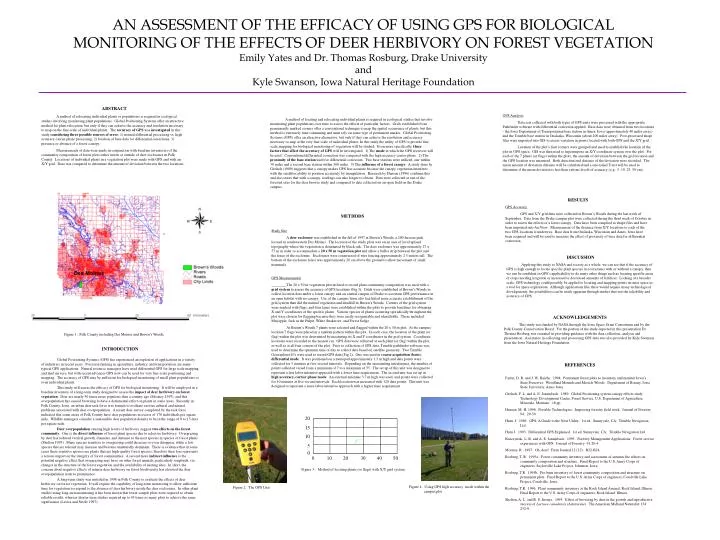
20 15 10 5 0 0 10 20 30 40 50 Figure 3 : Method of locating plants (or flags) with X/Y grid system. Figure 4: Using GPS high accuracy mode within the campus plot. Figure 2: The GPS Unit. AN ASSESSMENT OF THE EFFICACY OF USING GPS FOR BIOLOGICAL MONITORING OF THE EFFECTS OF DEER HERBIVORY ON FOREST VEGETATIONEmily Yates and Dr. Thomas Rosburg, Drake Universityand Kyle Swanson, Iowa Natural Heritage Foundation ABSTRACT A method of relocating individual plants or populations is required in ecological studies involving monitoring plant populations. Global Positioning Systems offer an attractive method for plant relocation, but only if they can achieve the accuracy and resolution necessary to map on the fine scale of individual plants. The accuracy of GPS was investigated in this study considering three possible sources of error: 1) normal differential processing vs. high accuracy carrier phase processing, 2) location of base data for differential corrections, 3) presence or absence of a forest canopy. Measurements of data were made in conjunction with baseline inventories of the community composition of forest plots either inside or outside of deer exclosures in Polk County. Locations of individual plants in a vegetation plot were made with GPS and with an X/Y grid. Data was compared to determine the amount of deviation between the two locations. GPS Analysis Data sets collected with both types of GPS units were processed with the appropriate Pathfinder software with differential correction applied. Base data were obtained from two locations - the Iowa Department of Transportation base station in Ames, Iowa (approximately 40 miles away) and the Trimble base station in Onalaska, Wisconsin (about 200 miles away). Post-processed shape files were imported into GIS to assess variation in points located with both GPS and the X/Y grid. Location of the plot’s four corners were grouped and used to establish the location of the plot in GPS space. GIS was then used to superimpose an X/Y coordinate system over the plot. For each of the 7 plants (or flags) within the plots, the amount of deviation between the grid location and the GPS location was measured. Both direction and distance of the deviation were recorded. The mean amount of deviation distance will be calculated and a one-tailed T-test will be used to determine if the mean deviation is less than various levels of accuracy (e.g., 5, 10, 25, 50 cm). A method of locating and relocating individual plants is required in ecological studies that involve monitoring plant populations over time to assess the effects of particular factors. Grids established from permanently marked corners offer a conventional technique to map the spatial occurrence of plants, but this method is extremely time consuming and must rely on some type of permanent marker. Global Positioning Systems (GPS) offer an attractive alternative, but only if they can achieve the resolution and accuracy necessary to map at the very fine scale of individual plants. In this study the utility of GPS to provide fine scale mapping for biological monitoring of vegetation will be studied. Even more specifically, three factors that affect the accuracy of GPS will be investigated. 1) The mode in which the GPS receivers will be used. Conventional differential correction was compared with the high accuracy carrier phase. 2) The proximity of the base station used for differential correction. Two base stations were utilized, one within 50 miles and a second base station within 300 miles. 3) The influence of a forest canopy. A study done by Gerlach (1989) suggests that a canopy makes GPS less accurate because the canopy vegetation interferes with the satellites ability to position accurately by triangulation. Research by Hansen (1996) confirms this and also states that with a canopy, readings can take longer to obtain. Data were collected at one of the forested sites for the deer browse study and compared to data collected on an open field on the Drake campus. INTRODUCTION Global Positioning Systems (GPS) has experienced an explosion of applications in a variety of industries in recent years. Precision farming in agriculture, industry, and transportation are many typical GPS applications. Natural resource managers have used differential GPS for large scale mapping and land surveys, but with recent advances GPS now can be used for very fine scale positioning and mapping. The accuracy of GPS may be sufficient for biological monitoring of small plant populations or even individual plants. This study will assess the efficacy of GPS for biological monitoring. It will be employed in a baseline inventory of a long-term study designed to assess the impact of deer herbivory on forest vegetation. Deer are nearly 50 times more populous than a century ago (Mooney 1997), and this overpopulation has caused browsing to have a detrimental effect on plants in some areas. Recently in Polk County, Iowa, an urban deer task force was formed to evaluate various cultural and natural problems associated with deer overpopulation. A recent deer survey completed by the task force indicated that some areas of Polk County have deer populations in excess of 170 individuals per square mile. Wildlife managers consider a sustainable deer population density to be in the range of 8 to 15 deer per square mile. Deer overpopulation causing high levels of herbivory suggest two effects on the forest community. One is the direct influence of forest plant species due to selective herbivory. Overgrazing by deer has reduced vertical growth, diameter, and distance to the next species in species of forest plants (Shelton 1995). Many species sensitive to overgrazing could decrease or even disappear, while a few species that are tolerant may increase and become unnaturally dominant. There is evidence that in some cases these sensitive species are plants that are high-quality forest species; therefore their loss represents a serious impact on the integrity of forest communities. A second more indirect influence is the potential negative effect that overgrazing may have on other forest animals, particularly songbirds, via changes in the structure of the forest vegetation and the availability of nesting sites. In short, the concern about negative effects of intense deer herbivory on forest biodiversity has elevated the deer overpopulation issue to prominence. A long-term study was initiated in 1998 in Polk County to evaluate the effects of deer herbivory on forest vegetation. It will require the capability of long-term monitoring to allow sufficient time for vegetation to respond to the absence of deer herbivory inside the deer exclosures. In other plant studies using long-term monitoring it has been shown that fewer sample plots were required to obtain reliable results, whereas shorter term studies required up to 45 times as many plots to achieve the same significance (Lesica and Steele 1997). RESULTS GPS Accuracy GPS and X/Y grid data were collected at Brown’s Woods during the last week of September. Data from the Drake campus plot were collected during the third week of October in order to assess the effects of a forest canopy. Data have been compiled as shape files and have been imported into ArcView. Measurement of the distance from X/Y locations to each of the two GPS locations is underway. Base data from Onalaska, Wisconsin and Ames, Iowa have been acquired and will be used to measure the effect of proximity of base data for differential correction. METHODS Study Site A deer exclosure was established in the fall of 1997 at Brown’s Woods, a 200-hectare park located in southwestern Des Moines. The location of the study plots was on an area of level upland topography where the vegetation is dominated by black oak. The deer exclosure was approximately 27 x 57 m in order to accommodate a 20 x 50 m vegetation plot and allow a buffer strip between the plot and the fence of the exclosure. Exclosures were constructed of wire fencing approximately 2.5 meters tall. The bottom of the exclosure fence was approximately 20 cm above the ground to allow movement of small mammals. GPS Measurements The 20 x 50 m vegetation plot utilized to record plant community composition was used with a grid system to assess the accuracy of GPS locations (Fig 3). Grids were established at Brown’s Woods to collect location data under a forest canopy and on central campus of Drake to ascertain GPS performance in an open habitat with no canopy. Use of the campus lawn also facilitated more accurate establishment of the grid system than did the natural vegetation and deadfall in Brown’s Woods. Corners of the grid system were marked with flags, and four lanes were established within the plots to provide baselines for obtaining X and Y coordinates of the specific plants. Various species of plants occurring sporadically throughout the plot were chosen for flagging because they were easily recognizable and identifiable. These included Mayapple, Jack in the Pulpit, White Snakeroot, and Forest Sedge. At Brown’s Woods 7 plants were selected and flagged within the 20 x 50 m plot. At the campus location 7 flags were placed in a random pattern within the plot. In each case, the location of the plant (or flag) within the plot was determined by measuring its X and Y coordinates in the grid system. Coordinate locations were recorded to the nearest cm. GPS data were collected at each plant (or flag) within the plot, as well as at all four corners of the plot. Prior to collection of GPS data, Trimble pathfinder software was used to determine the optimum time of day to collect data based on satellite geometry. Two Trimble Geoexplorer II’s were used to record GPS data (Fig 2). One was used in coarse acquisition (basic) differential mode. It was positioned on a monopod approximately 1.3 m high and data points were collected for 5 minutes at five-second intervals. Depending on the surrounding interference, the number of points collected varied from a minimum of 7 to a maximum of 55. The set up of this unit was designed to represent a less labor-intensive approach with a lower time requirement. The second unit was set up in high accuracy, carrier phase mode. An external antennae 3.7 m high was used, and points were collected for 10 minutes at five-second intervals. Each location was measured with 120 data points. This unit was designed to represent a more labor-intensive approach with a higher time requirement. DISCUSSION Applying this study to NASA and society as a whole, we can see that if the accuracy of GPS is high enough to locate specific plant species in ecosystems with or without a canopy, then we can be confident in GPS’s applicability to do many other things such as locating specific areas of crops needing irrigation or increased or decreased amounts of fertilizer. Looking at a broader scale, GPS technology could possibly be applied to locating and mapping points in outer space as a tool for space exploration. Although applications like these would require many technological developments, the possibilities can be made apparent through studies that test the reliability and accuracy of GPS. ACKNOWLEDGEMENTS This study was funded by NASA through the Iowa Space Grant Consortium and by the Polk County Conservation Board. For the portion of the study depicted in this presentation Dr. Thomas Rosburg was essential in providing guidance with the data collection, analysis and presentation. Assistance in collecting and processing GPS data was also provided by Kyle Swanson from the Iowa Natural Heritage Foundation. Figure 1: Polk County including Des Moines and Brown’s Woods. REFERENCES Farrar, D. R. and J. W. Raiche. 1994. Permanent forest plots to inventory and monitor Iowa’s State Preserves: Woodland Mounds and Mericle Woods. Department of Botany, Iowa State University, Ames Iowa. Gerlach, F. L. and A. E. Jasumback. 1989. Global Positioning system canopy effects study. Technology Development Center, Forest Service, U.S. Department of Agriculture, Missoula, Montana. 18 pp. Hansen, M. H. 1996. Portable Technologies: Improving forestry field work. Journal of Forestry 94: 29-30. Hurn, J. 1989. GPS: A Guide to the Next Utility. 1st ed. Sunnyvale, CA: Trimble Navigation Ltd. Hurn J. 1993. Differential GPS Explained. 1st ed. Sunnyvale, CA: Trimble Navigation Ltd. Kruczynski, L. R. and A. E. Jasumback. 1993. Forestry Management Applications: Forest service experiences with GPS. Journal of Forestry 91:20-4. Mooney, R. 1997. Oh, deer! Farm Journal 12 (12): B22-B24. Rosburg, T. R. 1995a. Forest community inventory and assessment of autumn fire effects on community composition and structure. Final Report to the U.S. Army Corps of engineers, Saylorville Lake Project, Johnston, Iowa. Rosburg, T.R. 1995b. Pre-burn inventory of forest community composition and structure on permanent plots. Final Report to the U.S. Army Corps of engineers, Coralville Lake Project, Coralville, Iowa. Rosburg, T.R. 1996. Plant community inventory at the Rock Island Arsenal, Rock Island, Illinois. Final Report to the U.S. Army Corps of engineers, Rock Island, Illinois. Shelton, A. L. and R. S. Inouye. 1995. Effect of browsing by deer in the growth and reproductive success of Lactuca canadensis (Asteraceae). The American Midland Naturalist 134: 232-9.