Download
1 / 31
310 likes | 909 Vues
Pattern Classification All materials in these slides were taken from Pattern Classification (2nd ed) by R. O. Duda, P. E. Hart and D. G. Stork, John Wiley & Sons, 2000 with the permission of the authors and the publisher. Chapter 3: Maximum-Likelihood and Bayesian Parameter Estimation (part 2).

E N D
Pattern ClassificationAll materials in these slides were taken fromPattern Classification (2nd ed) by R. O. Duda, P. E. Hart and D. G. Stork, John Wiley & Sons, 2000with the permission of the authors and the publisher Pattern Classification, Chapter 3
Chapter 3:Maximum-Likelihood and Bayesian Parameter Estimation (part 2) • Bayesian Estimation (BE) • Bayesian Parameter Estimation: Gaussian Case • Bayesian Parameter Estimation: General Estimation • Problems of Dimensionality • Computational Complexity • Component Analysis and Discriminants • Hidden Markov Models
Bayesian Estimation (Bayesian learning to pattern classification problems) • In MLE was supposed fix • In BE is a random variable • The computation of posterior probabilities P(i | x) lies at the heart of Bayesian classification • Goal: compute P(i | x, D) Given the sample D, Bayes formula can be written Pattern Classification, Chapter 3 3
To demonstrate the preceding equation, use: Pattern Classification, Chapter 3 3
Bayesian Parameter Estimation: Gaussian Case Goal: Estimate using the a-posteriori density P( | D) • The univariate case: P( | D) is the only unknown parameter (0 and 0 are known!) Pattern Classification, Chapter 3 4
But we know Plugging in their gaussian expressions and extracting out factors not depending on m yields: Pattern Classification, Chapter 3 4
Observation: p(m|D) is an exponential of a quadratic It is again normal! It is called a reproducing density Pattern Classification, Chapter 3 4
Identifying coefficients in the top equation with that of the generic Gaussian Yields expressions for mn and sn2 Pattern Classification, Chapter 3 4
Solving for mn and sn2 yields: From these equations we see as n increases: • the variance decreases monotonically • the estimate of p(m|D) becomes more peaked Pattern Classification, Chapter 3 4
The univariate case P(x | D) • P( | D) computed (in preceding discussion) • P(x | D) remains to be computed! It provides: We know s2 and how to compute (Desired class-conditional density P(x | Dj, j)) Therefore: using P(x | Dj, j) together with P(j) And using Bayes formula, we obtain the Bayesian classification rule: Pattern Classification, Chapter 3 4
3.5 Bayesian Parameter Estimation: General Theory • P(x | D) computation can be applied to any situation in which the unknown density can be parameterized: the basic assumptions are: • The form of P(x | ) is assumed known, but the value of is not known exactly • Our knowledge about is assumed to be contained in a known prior density P() • The rest of our knowledge is contained in a set D of n random variables x1, x2, …, xn that follows P(x) Pattern Classification, Chapter 3 5
The basic problem is: “Compute the posterior density P( | D)” then “Derive P(x | D)”, where Using Bayes formula, we have: And by the independence assumption: Pattern Classification, Chapter 3 5
Convergence (from notes) Pattern Classification, Chapter 3
Problems of Dimensionality • Problems involving 50 or 100 features are common (usually binary valued) • Note: microarray data might entail ~20000 real-valued features • Classification accuracy dependant on • dimensionality • amount of training data • discrete vs continuous Pattern Classification, Chapter 3 7
Case of two class multivariate normal with the same covariance • P(x|j) ~N(j,), j=1,2 • Statistically independent features • If the priors are equal then: Pattern Classification, Chapter 3 7
If features are conditionally independent then: • Do we remember what conditional independence is? • Example for binary features: Let pi= Pr[xi=1|1] then P(x|1) is the product of the pi Pattern Classification, Chapter 3 7
Most useful features are the ones for which the difference between the means is large relative to the standard deviation • Doesn’t require independence • Adding independent features helps increase r reduce error • Caution: adding features increases cost & complexity of feature extractor and classifier • It has frequently been observed in practice that, beyond a certain point, the inclusion of additional features leads to worse rather than better performance: • we have the wrong model ! • we don’t have enough training data to support the additional dimensions Pattern Classification, Chapter 3 7
7 7 Pattern Classification, Chapter 3 7
Computational Complexity • Our design methodology is affected by the computational difficulty • “big oh” notation f(x) = O(h(x)) “big oh of h(x)” If: (An upper bound on f(x) grows no worse than h(x) for sufficiently large x!) f(x) = 2+3x+4x2 g(x) = x2 f(x) = O(x2) Pattern Classification, Chapter 3 7
“big oh” is not unique! f(x) = O(x2); f(x) = O(x3); f(x) = O(x4) • “big theta” notation f(x) = (h(x)) If: f(x) = (x2) but f(x) (x3) Pattern Classification, Chapter 3 7
Complexity of the ML Estimation • Gaussian priors in d dimensions classifier with n training samples for each of c classes • For each category, we have to compute the discriminant function Total = O(d2n) Total for c classes = O(cd2n) O(d2n) • Cost increase when d and n are large! Pattern Classification, Chapter 3 7
Overfitting • Dimensionality of model vs size of training data • Issue: not enough data to support the model • Possible solutions: • Reduce model dimensionality • Make (possibly incorrect) assumptions to better estimate Pattern Classification, Chapter 3
Overfitting • Estimate better • use data pooled from all classes • normalization issues • use pseudo-Bayesian form 0 + (1-)n • “doctor” by thresholding entries • reduces chance correlations • assume statistical independence • zero all off-diagonal elements Pattern Classification, Chapter 3
Shrinkage • Shrinkage: weighted combination of common and individual covariances • We can also shrink the estimate common covariances toward the identity matrix Pattern Classification, Chapter 3
Component Analysis and Discriminants • Combine features in order to reduce the dimension of the feature space • Linear combinations are simple to compute and tractable • Project high dimensional data onto a lower dimensional space • Two classical approaches for finding “optimal” linear transformation • PCA (Principal Component Analysis) “Projection that best represents the data in a least- square sense” • MDA (Multiple Discriminant Analysis) “Projection that best separatesthe data in a least-squares sense” Pattern Classification, Chapter 3 8
PCA (from notes) Pattern Classification, Chapter 3
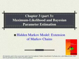
Hidden Markov Models: • Markov Chains • Goal: make a sequence of decisions • Processes that unfold in time, states at time t are influenced by a state at time t-1 • Applications: speech recognition, gesture recognition, parts of speech tagging and DNA sequencing, • Any temporal process without memory T = {(1), (2), (3), …, (T)} sequence of states We might have 6 = {1, 4, 2, 2, 1, 4} • The system can revisit a state at different steps and not every state need to be visited Pattern Classification, Chapter 3 10
First-order Markov models • Our productions of any sequence is described by the transition probabilities P(j(t + 1) | i (t)) = aij Pattern Classification, Chapter 3 10
= (aij, T) P(T |) = a14 . a42 . a22 . a21 . a14 . P((1) = i) Example: speech recognition “production of spoken words” Production of the word: “pattern” represented by phonemes /p/ /a/ /tt/ /er/ /n/ // ( // = silent state) Transitions from /p/ to /a/, /a/ to /tt/, /tt/ to er/, /er/ to /n/ and /n/ to a silent state Pattern Classification, Chapter 3 10