Download
1 / 16
160 likes | 172 Vues
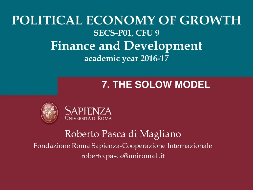
POLITICAL ECONOMY OF GROWTH SECS-P01, CFU 9 Finance and Development academic year 2016-17. 7. THE SOLOW MODEL. Roberto Pasca di Magliano Fondazione Roma Sapienza-Cooperazione Internazionale roberto.pasca@uniroma1.it. Model Background.

E N D
POLITICAL ECONOMY OF GROWTHSECS-P01, CFU 9Finance and Developmentacademic year 2016-17 7. THE SOLOW MODEL Roberto Pasca di Magliano Fondazione Roma Sapienza-Cooperazione Internazionale roberto.pasca@uniroma1.it
Model Background The Solow growth model is the starting point to determine why growth differs across similar countries it builds on the Cobb-Douglas production model by adding a theory of capital accumulation developed in the mid-1950s by Robert Solow of MIT, it is the basis for the Nobel Prize he received in 1987 the accumulation of capital is a possible engine of long-run economic growth
Building the Model: goods market supply We begin with a production function and assume constant returns. Y=F(K,L) so… zY=F(zK,zL) By setting z=1/L it is possible to create a per worker function. Y/L=F(K/L,1) So, output per worker is a function of capital per worker. y=f(k)
Building the Model: goods market supply y y=f(k) k • The slope of this function is the marginal product of capital per worker.MPK = f(k+1)–f(k) • It tells us the change in output per worker that results when we increase the capital per worker by one. Change in y Change in k
Building the Model:goods market demand Begining with per worker consumption and investment (Government purchases and net exports are not included in the Solow model), the following per worker national income accounting identity can be obtained: y = c+I Given a savings rate (s) and a consumption rate (1–s) a consumption function can generated:c = (1–s)y …which is the identity. Theny = (1–s)y + I …rearranging,i = s*y …so investment per worker equals savings per worker.
Steady State Equilibrium The Solow model long run equilibrium occurs at the point where both (y) and (k) are constant. The endogenous variables in the model are y and k. The exogenous variable is (s).
Steady State Equilibrium In order to reach the stady state equilibrium: By substituting f(k) for (y), the investment per worker function (i = s*y) becomes a function of capital per worker (i = s*f(k)). By adding a depreciation rate (d). The impact of investment and depreciation on capital can be developed to evaluate the need of capital change: dk = i – dk …substituting for (i) dk = s*f(k) – dk
Investment, Depreciation At this point, dKt = sYt, so Capital, Kt The Solow Diagram equilibriumproduction function, capital accumulation (Kt on the x-axis)
Depreciation: d K Investment: s Y Investment, depreciation Net investment K0 K* Capital, K The Solow DiagramWhen investment is greater than depreciation, the capital stock increase until investment equals depreciation. At this steady state point, dK = 0
Investment, Depreciation K0 K1 Capital, Kt Suppose the economy starts at K0: • The red line is above the green at K0: • Saving = investment is greater than depreciation at K0 • So ∆Kt > 0 because • Since ∆Kt >0, Kt increases from K0 to K1 > K0
Investment, Depreciation K0 K1 Capital, Kt Now imagine if we start at a K0 here: • At K0, the green line is above the red line • Saving = investment is now less thandepreciation • So ∆Kt < 0 because • Then since ∆Kt<0,Ktdecreases from K0 to K1 < K0
Investment, Depreciation No matter where we start, we’ll transition to K*! At this value of K, dKt = sYt, so K* Capital, Kt We call this the process of transition dynamics: Transitioning from any Kt toward the economy’s steady-state K*, where ∆Kt = 0 and growth ceases
Changing the exogenous variable - savings Investment, Depreciation dk s*f(k) s*f(k*)=dk* k k* • We know that steady state is at the point where s*f(k)=dk s*f(k*)=dk* s*f(k) • What happens if we increase savings? • This would increase the slope of our investment function and cause the function to shift up. k** • This would lead to a higher steady state level of capital. • Similarly a lower savings rate leads to a lower steady state level of capital.
Y* K* We can see what happens to output, Y, and thus to growth if we rescale the vertical axis: Investment, Depreciation, Income • Saving = investment and depreciation now appear here • Now output can be graphed in the space above in the graph • We still have transition dynamics toward K* • So we also have dynamics toward a steady-state level of income, Y* Capital, Kt
Investment, depreciation, and output Y0 Y* Investment: s Y Depreciation: d K Consumption K0 K* Capital, K The Solow Diagram with OutputAt any point, Consumption is the difference between Output and Investment: C = Y – I Output: Y
Conclusion The Solow Growth model is a dynamic model that allows us to see how our endogenous variables capital per worker and output per worker are affected by the exogenous variable savings. We also see how parameters such as depreciation enter the model, and finally the effects that initial capital allocations have on the time paths toward equilibrium. In other section the dynamic model is improved in order to include changes in other exogenous variables; population and technological growth.