Download
1 / 35
350 likes | 362 Vues
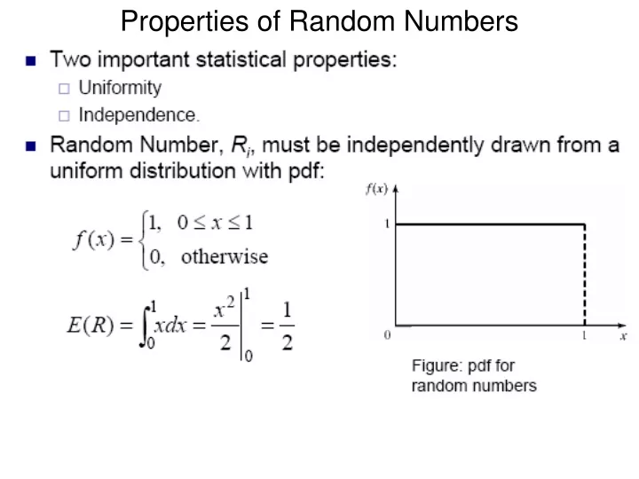
Properties of Random Numbers. Consequences of Uniformity and Independence Properties: Expected no. of observations in each interval = N/n The probability of observing a particular interval is independent of the previous values drawn.

E N D
Consequences of Uniformity and Independence Properties: • Expected no. of observations in each interval = N/n • The probability of observing a particular interval is independent of the previous values drawn.
“Pseudo”, because generating numbers using a known method removes the potential for true randomness. • Important considerations in RN routines: • Fast • Portable to different computers • Have sufficiently long cycle : the length of the sequence of RNs before the • previous nos begin to repeat themselves in an earlier order. • Replicable (from given starting point) • Closely approximate the ideal statistical properties of uniformity and independence. Generation of Pseudo-Random Numbers • Techniques for Generating Random Numbers • Linear Congruential Method (LCM). • Combined Linear Congruential Generators (CLCG).
Linear Congruential Method If c ≠ 0, Mixed congruential method If c=0 , Multiplicative congruential method
Maximum Density : • means that the values assumed by Ri, i = 1,2,…, leave no large gaps on [0,1] • Maximum Period: • To achieve maximum density and avoid cycling. • Achieved by: proper choice of a, c, m, and X0. • Rules: Characteristics of a Good Generator
Example: For 32-bit computers,L’Ecuyer suggests combining k=2 generators with m1=2147483563, a1= 40014, m2=2147483399 and a2=40692. Algorithm: • Select seed X1,0 in the range [1, 2147483563] for the first generator and seed X2,0 in the range [1, 2147483399] for the second generator. Set j=0 • Evaluate each individual generator. X1,j+1 = 40014 X1,j+1 mod 2147483563 X2,j+1 = 40692 X2,j+1 mod 2147483399 • Set Xj+1 =(X1,j+1 - X2,j+1 ) mod 2147483562 • Return Rj+1 = Xj+1 / 2147483563 , Xj+1>0 2147483562 / 2147483563 , Xj+1=0 5. Set j=j+1 and go to step 2. Period =(m1-1)(m2-1)/2
If several tests are conducted on the same set of numbers, the probability of rejecting null hypothesis on at lest one test by chance alone increases. • Similarly if one test is conducted on many sets of numbers, the probability of rejecting null hypothesis on at least one test by chance alone increases.
These tests are based on the null hypothesis of no significant difference between sample distribution and the theoretical distribution. Frequency Tests
Kolmogorov-Smirnov test :Steps Step 1: Rank the data from smallest to largest. Let R(i) denote the ith smallest observation , so that R(1)≤ R(2) ≤………..≤R(N) Step 2: Compute Step 3: Compute D= max(D+, D-) Step 4: Determine the critical value Dαfrom Table A.8 for the specified significance level α and the given sample size N. Step 5: If the sample statistic D > Dα, the null hypothesis is rejected. If D≤ Dα, conclude that no difference has been detected between the true distribution of {R1,R2,…….RN} and the uniform distribution.
2. Chi-square test Notes: It is recommended that n and N should be chosen so that each Ei >= 5 Degrees of freedom: the number of values in the final calculation of the statistic that are free to vary. DOF= [ No of independent pieces that go into estimate] – [No of para estimated as inermediate steps in the estimation of para itself]
II . Runs Tests This test examines the arrangement of nos in a sequence to test the hypothesis of independence. Run: A succession of similar events preceded and followed by a different event. Length of the run: No of events that occur in the run. Ex. H T T H H T T T H T No of runs: 06 Lengths: 1 2 2 3 1 1 Two Possible Concerns: 1. No. of Runs 2. Length of runs
Runs up and runs down: • Up run: a sequence of numbers each of which is succeeded by a larger no. • Down run: a sequence of numbers each of which is succeeded by a smaller no. • Ex: 0.87 0.15 0.23 0.45 0.69 0.32 0.30 0.19 0.24 0.18 0.65 0.82 0.93 0.22 0.81 -0.87 +0.15 +0.23 +0.45 -0.69 -0.32 -0.30 +0.19 -0.24 +0.18 +0.65 +0.82 -0.93 +0.22 0.81 - + + + - - - + - + + + - + Sequence of +’s and –’s forms a run . No of runs=8 = 4 up + 4 down
If a is total no. of runs in a random sequence, For N>20, a ~ N(μa, σa2 ) In this case, Test Statistics is where Z0 ~N(0,1) Failure to reject the hypothesis of independence occurs when –zα/2 ≤ Z0 ≤ zα/2
+ 2.Runs above and below the mean: Let n1= No. of observations above the mean and n2= No. of observations below the mean (0.99+0.00)/2=0.495 Given n1 and n2 , the mean and variance of b( total no of runs)for a truly independent sequence are given by: μb= 2n1n2 1 and σb2 = 2n1n2 (2n1n2 - N) N 2 N2 (N-1) For either n1 or n2 > 20 , b ~ N(μb, σb2 ). Test statistics: • Failure to reject the hypothesis of independence occurs when –z α/2 ≤ Z0 ≤ z α/2
3. Runs Test: length of runs: Let Yi be the no of runs of length i in a sequence of N nos. For an independent sequence , the E(Yi ) for runs up and down is given by E(Yi ) = 2 [N(i2 +3i +1)- (i3 + 3i2-i-4)], i<= N-2 (i+3)! =2 , i = N - 1 N! For runs above and below mean: E(Yi ) = Nwi , N> 20 E(I) where wi , is approx. prob that a run has length i wi = (n1/N)i (n2/N) + (n1/N)(n2/N)i , N > 20 and E(I) is appro. expected length of run E(I) = (n1/n2) + (n2/n1) , N>20
The approx. expected total no. of runs (of all the lengths) in a sequence of length N is: E(A) = N / E(I) , N>20 The appropriate test is Chi-square test with Oi being the observed no of runs of length i . Test statistics : X0 2 = ∑ {[Oi- E(Yi) ] 2 / E(Yi)}, i = 1 to L where L = N-1 for runs up and down L = N for runs above and below mean If H0 of independence is true then X0 2 is approx. Chi-square distributed with L-1 degrees of freedom.
III. Gap Test Used to determine the significance of interval between the recurrences of the same digit. Ex. 4 1 3 5 1 7 2 8 2 0 7 9 1 3 5 2 7 9 4 1 6 33 9 6 3 4 8……….. Frequency of gaps is of interest . Prob of 1st gap :P(gap of 10)= P(no 3)……..P(no 3) P(3) = (0.9)10 (0.1) In general, P( t followed by exactly x non-t digits) = (0.9)x (0.1)
Theoretical distribution for randomly ordered digits is given by P(gap<=x) = F(x) = 0.1 ∑ (0.9) n for n=0 to x = 1 – (0.9) x+1 Steps: Specify the cdf for theoretical frequency distribution based on the selected class interval width. Arrange the observed sample of gaps in a cumulative distribution with these same classes. Find D , max deviation between SN(x) and F(x). D = max |F(x) - SN(x)| Determine the critical value Dα form table A.8 for specified value of α and sample size,N. If D > Dα , Ho of independence is rejected. Note: The no. of gaps = No. of data values – No. Of distinct digits
IV. Poker Test It is based on the frequency with which certain digits are repeated in a series of numbers. Uses Chi square statistics. If we consider 3- digit nos, there are only 3 possibilities: 1. The individual nos can all be different. 2. The individual nos can all be same. 3. There can be one pair of like digits. P(3 different digits) = P(2nd different from first) x P(3rd different from 1st and 2nd) = (0.9) (0.8) = 0.72 P(3 like digits)= P(2nd same as first) x P(3rd same as 1st ) = (0.1) (0.1) = 0.1 P(exactly one pair) = 1 - 0.72 - 0.1 = 0.27
Example: A sequence of 1000 3-digit nos has been generated and an analysis indicates that 680 have 3 different digits, 289 contain exactly one pair of like digits and 31 contain 3 like digits. Based on Poker test , are these nos independent? (α = 0.05) Solution:
Test is concerned with the dependence between the numbers in a sequence. • It tests the correlation between the numbers and compares the sample correlation to expected correlation of zero. • Test require the computaion of autocorrelation ρim between every m numbers starting with ith no. Ri, Ri+m, Ri+2m, …………..,R i+(M+1)m The value M is the largest integer such that i+(M+1)m <=N • H0: ρim = 0 H1: ρim ≠ 0 V .Tests for Autocorrelation
After computing Z0, do not reject the null hypothesis of independence if –Zα/2 <= Z0<= Zα/2