Download
1 / 23
260 likes | 540 Vues
Inventory Management and Risk Pooling (1). Designing & Managing the Supply Chain Chapter 3 Byung-Hyun Ha bhha@pusan.ac.kr. Outline. Introduction to Inventory Management The Effect of Demand Uncertainty (s,S) Policy Supply Contracts Periodic Review Policy Risk Pooling

E N D
Inventory Management and Risk Pooling (1) Designing & Managing the Supply Chain Chapter 3 Byung-Hyun Ha bhha@pusan.ac.kr
Outline • Introduction to Inventory Management • The Effect of Demand Uncertainty • (s,S) Policy • Supply Contracts • Periodic Review Policy • Risk Pooling • Centralized vs. Decentralized Systems • Practical Issues in Inventory Management
Case: JAM USA, Service Level Crisis • Background • Subsidiary of JAM Electronics (Korean manufacturer) • Established in 1978 • Five Far Eastern manufacturing facilities, each in different countries • 2,500 different products, a central warehouse in Korea for FGs • A central warehouse in Chicago with items transported by ship • Customers: distributors & original equipment manufacturers (OEMs) • Problems • Significant increase in competition • Huge pressure to improve service levels and reduce costs • Al Jones, inventory manage, points out: • Only 70% percent of all orders are delivered on time • Inventory, primarily that of low-demand products, keeps pile up
Case: JAM USA, Service Level Crisis • Reasons for the low service level: • Difficulty forecasting customer demand • Long lead time in the supply chain • About 6-7 weeks • Large number of SKUs handled by JAM USA • Low priority given the U.S. subsidiary by headquarters in Seoul Monthly demand for item xxx-1534
Inventory • Where do we hold inventory? • Suppliers and manufacturers / Warehouses and distribution centers / Retailers • Types of Inventory • WIP (work in process) / raw materials / finished goods • Reasons of holding inventory • Unexpected changes in customer demand • The short life cycle of an increasing number of products. • The presence of many competing products in the marketplace. • Uncertainty in the quantity and quality of the supply, supplier costs and delivery times. • Delivery Lead Time, Capacity limitations • Economies of scale (transportation cost)
Key Factors Affecting Inventory Policy • Customer demand Characteristics • Replenishment lead Time • Number of Products • Service level requirements • Cost Structure • Order cost • Fixed, variable • Holding cost • Taxes, insurance, maintenance, handling, obsolescence, and opportunity costs • Objectives: minimize costs
EOQ: A View of Inventory • Assumptions • Constant demand rate of D items per day • Fixed order quantities at Q items per order • Fixed setup cost K when places an order • Inventory holding cost h per unit per day • Zero lead time • Zero initial inventory & infinite planning horizon
EOQ: A View of Inventory • Inventory level • Total inventory cost in a cycle of length T • Average total cost per unit of time (Q) Cycle time (T)
EOQ: A View of Inventory • Trade-off between order cost and holding cost Total Cost Holding Cost Order Cost
EOQ: A View of Inventory • Optimal order quantity • Important insights • Tradeoff between set-up costs and holding costs when determining order quantity. In fact, we order so that these costs are equal per unit time • Total cost is not particularly sensitive to the optimal order quantity
The Effect of Demand Uncertainty • Most companies treat the world as if it were predictable: • Production and inventory planning are based on forecasts of demand made far in advance of the selling season • Companies are aware of demand uncertainty when they create a forecast, but they design their planning process as if the forecast truly represents reality • Recent technological advances have increased the level of demand uncertainty: • Short product life cycles • Increasing product variety • Three principles of all forecasting techniques: • Forecasting is always wrong • The longer the forecast horizon the worst is the forecast • Aggregate forecasts are more accurate
Case: Swimsuit Production • Fashion items have short life cycles, high variety of competitors • Swimsuit production • New designs are completed • One production opportunity • Based on past sales, knowledge of the industry, and economic conditions, the marketing department has a probabilistic forecast • The forecast averages about 13,000, but there is a chance that demand will be greater or less than this
Case: Swimsuit Production • Information • Production cost per unit (C): $80 • Selling price per unit (S): $125 • Salvage value per unit (V): $20 • Fixed production cost (F): $100,000 • Q is production quantity
Case: Swimsuit Production • Scenario One: • Suppose you make 10,000 swimsuits and demand ends up being 12,000 swimsuits. • Profit = 125(10,000) - 80(10,000) - 100,000 = $350,000 • Scenario Two: • Suppose you make 10,000 swimsuits and demand ends up being 8,000 swimsuits. • Profit = 125(8,000) - 80(10,000) - 100,000 + 20(2,000) = $140,000
Swimsuit Production Solution • Find order quantity that maximizes weighted average profit • Question: Will this quantity be less than, equal to, or greater than average demand? • Average demand is 13,000 • Look at marginal cost vs. marginal profit • if extra swimsuit sold, profit is 125-80 = 45 • if not sold, cost is 80-20 = 60 • In case of Scenario Two (make 10,000, demand 8,000) • Profit = 125(8,000) - 80(10,000) - 100,000 + 20(2,000) = 45(8,000) - 60(2,000) - 100,000 = $140,000 • So we will make less than average
Swimsuit Production Solution • Quantity that maximizes average profit
Swimsuit Production Solution • Tradeoff between ordering enough to meet demand and ordering too much • Several quantities have the same average profit • Average profit does not tell the whole story • Question: 9000 and 16000 units lead to about the same average profit, so which do we prefer?
Swimsuit Production Solution • Risk and reward Consult Ch13 of Winston, “Decision making under uncertainty”
Case: Swimsuit Production • Key insights • The optimal order quantity is not necessarily equal to average forecast demand • The optimal quantity depends on the relationship between marginal profit and marginal cost • As order quantity increases, average profit first increases and then decreases • As production quantity increases, risk increases (the probability of large gains and of large losses increases)
Case: Swimsuit Production • Initial inventory • Suppose that one of the swimsuit designs is a model produced last year • Some inventory is left from last year • Assume the same demand pattern as before • If only old inventory is sold, no setup cost • Question: If there are 5,000 units remaining, what should Swimsuit production do?
Case: Swimsuit Production • Analysis for initial inventory and profit • Solid line: average profit excluding fixed cost • Dotted line: same as expected profit including fixed cost • Nothing produced • 225,000 (from the figure) + 80(5,000) = 625,000 • Producing • 371,000 (from the figure) + 80(5,000) = 771,000 • If initial inventory was 10,000?
Case: Swimsuit Production • Initial inventory and profit
Case: Swimsuit Production • (s, S) policies • For some starting inventory levels, it is better to not start production • If we start, we always produce to the same level • Thus, we use an (s, S) policy • If the inventory level is below s, we produce up to S • s is the reorder point, and S is the order-up-to level • The difference between the two levels is driven by the fixed costs associated with ordering, transportation, or manufacturing