Download
1 / 14
160 likes | 354 Vues
Rayleigh Bernard Convection and the Lorenz System During the last century there were three revolutions in Physics: General Relativity, Quantum Mechanics and Chaos. Low dimensional chaos applications range from atmospheric physics, to astronomy,

E N D
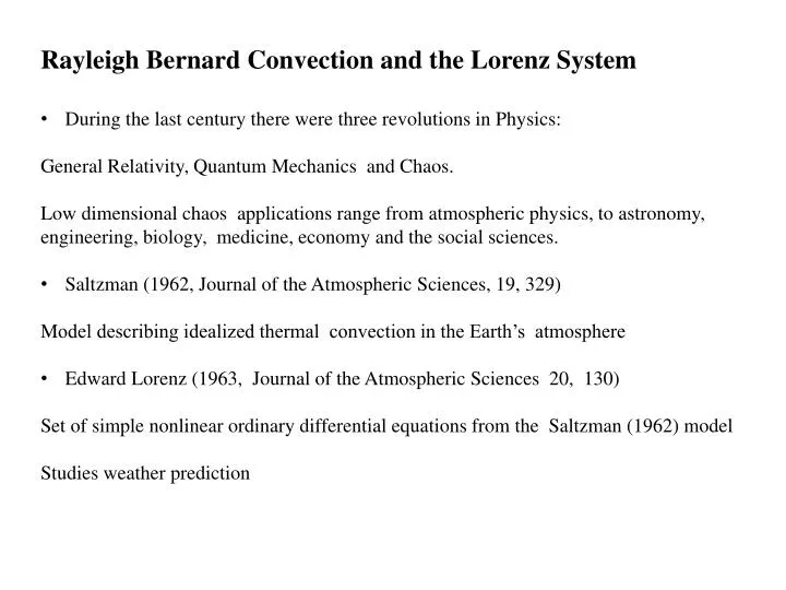
Rayleigh Bernard Convection and the Lorenz System • During the last century there were three revolutions in Physics: • General Relativity, Quantum Mechanics and Chaos. • Low dimensional chaos applications range from atmospheric physics, to astronomy, • engineering, biology, medicine, economy and the social sciences. • Saltzman (1962, Journal of the Atmospheric Sciences, 19, 329) • Model describing idealized thermal convection in the Earth’s atmosphere • Edward Lorenz (1963, Journal of the Atmospheric Sciences 20, 130) • Set of simple nonlinear ordinary differential equations from the Saltzman (1962) model • Studies weather prediction
Warm low density fluid rises Cool high density fluid sinks Fluid cools by loosing heat from the surface h a
Bénard Cells as seen by Meteosat-7 off the West Coast of Africa
Equations for Rayleigh Bernard convection after: Boussinesque approximation (ρ = constant except in gravity term) Writing in terms of dimensionless variables Πis the dimensionless pressure τ is the deviation of the temperature from linear behavior
After introducing the stream function ψ and combining equations (1) and (2) the pressure term is eliminated =0 z=0 z=h Ψ=0 at the boundary x=0 and x=a/h
Equations (4) and (5) without time dependence and non-linear terms Rayleigh conjectures a steady solution with this form where h is the height difference between the plates a is the horizontal width of the convections rolls The steady solutions satisfy the equations if the Rayleigh number has a critical vale
Salzman (1962) assumes a Lorenz transform to solve Equations 4 and 5. The time dependent coefficients Ψ and T are complex quantities
Attempting to match observations Salzman reduces the system by keeping components of Ψ1, Ψ2, T1 and T2 for wave numbers m , n 2 and for T2 m=0, n=(1,2,3,4). Ends with a system of coupled differential equations with 52 variables For the Prandtl number uses σ = 10 which is about twice the value for water (σ =4.8). Tries realistic values for R Chooses a = 6 h In the numerical experiments all but three of the variables tended to zero These three variables underwent irregular, non-periodic fluctuations
Inspired by Salzman, Lorenz (1963) makes the radical assumption that the solutions can be obtained if the series is truncated to include only 3 variables. Selects m=1, n=1 for the real parts of Ψ and T, and m=0, n=2 for the imaginary part of T:
With Lorenz’s assumption equations 4 and 5 radically simplify The non-linear terms in equation 5 all cancel and we are left with the simple system of three equations < --- From equation 5 < --- Two equations result from equation 4
Lorenz System: In addition to the Prandtl number σ, the factor r is the normalized Rayleigh number and b is a geometrical factor In his numerical experiments Lorenz used a= 1/ σ =10, b=8/3, r=28