Download
1 / 30
310 likes | 636 Vues
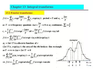
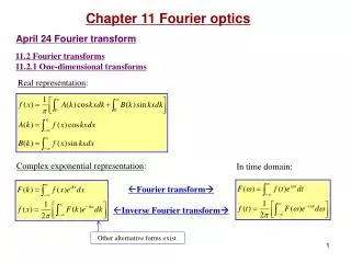
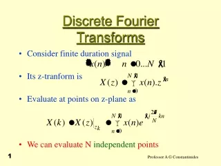
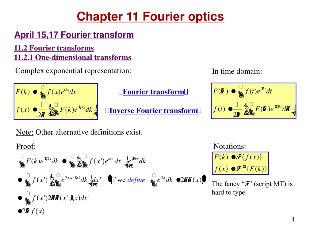
Chapter 11 Fourier optics. April 15,17 Fourier transform. 11.2 Fourier transforms 11.2.1 One-dimensional transforms. Complex exponential representation :. In time domain:. Note: Other alternative definitions exist. Notations:. Proof:. Fourier transform Inverse Fourier transform .

E N D
Chapter 11 Fourier optics April 15,17 Fourier transform 11.2 Fourier transforms 11.2.1 One-dimensional transforms Complex exponential representation: In time domain: Note: Other alternative definitions exist. Notations: Proof: Fourier transform Inverse Fourier transform The fancy “F” (script MT) is hard to type.
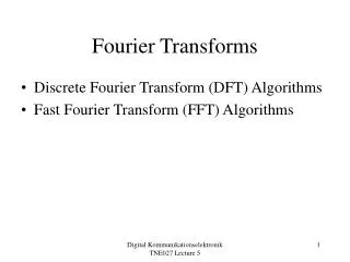
Example:Fourier transform of the Gaussian function 1) The Fourier transform of a Gaussian function is again a Gaussian function (self Fourier transform functions). 2) Standard deviations (where f (x) drops to e-1/2):
J0(u) J1(u) u
Read: Ch11: 1-2 Homework: Ch11: 2,3 Due: April 26
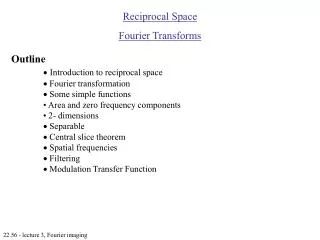
d (x) 1 x 0 d (x- x0) 1 x x0 0 April 19 Dirac delta function 11. 2.3 The Dirac delta function Dirac delta function: A sharp distribution function that satisfies: A way to show delta function Sifting property of the Dirac delta function: If we shift the origin, then
Delta sequence: A sequence that approaches the delta function when the distribution is gradually narrowed. The 2D delta function: The Fourier representation of delta function:
Displacement and phase shift: The Fourier transform of a function displaced in space is the transform of the undisplaced function multiplied by a linear phase factor. Proof:
Fourier transform of some functions: (constants, delta functions, combs, sines and cosines): f(x) F(k) f(x) F(k) 1 2p … x k x k 0 0 0 0 f(x) F(k) f(x) F(k) 1 1 … x k x 0 0 k 0 0
A(k) f(x) k x 0 f(x) B(k) k x 0 f(x) A(k) x k 0 f(x) B(k) k x 0
Read: Ch11: 2 Homework: Ch11: 4,8,10,11,12,17 Due: April 26
Z z Ii(Y,Z) I0(y,z) Y y April 22, 24 Convolution theorem 11.3 Optical applications 11.3.2 Linear systems Linear system: Suppose an object f (y, z) passing through an optical system results in an image g(Y, Z), the system is linear if 1) af (y, z) ag(Y, Z), 2) af1(y, z) + bf2(y, z) ag1(Y, Z) + bg2(Y, Z). We now consider the case of 1) incoherent light (intensity addible), and 2) MT = +1. The flux density arriving at the image point (Y, Z) from dydz is Point-spread function
z Z Ii(Y,Z) I0(y,z) y Y z Z I0(y,z) Ii(Y,Z) y Y Example: • The point-spread functionis the irradiance produced by the system with an input point source. In the diffraction-limited case with no aberration, the point-spread function is the Airy distribution function. • The image is the superposition of the point-spread function, weighted by the source radiant fluxes.
Space invariance: Shifting the object will only cause the shift of the image:
f(x) x h(x) x h(X-x) x X f(x)h(x) X 11.3.3 The convolution integral Convolution integral: The convolution integral of two functionsf (x) and h(x) is Symbol: g(X) = f(x)h(x) Example 1: The convolution of a triangular function and a narrow Gaussian function. Question: What is f(x-a)h(x-b)? Answer:
f(x) x h(x) x h(X-x) x X f(x)h(x) X Example 2: The convolution of two square functions. The convolution theorem: Proof: Example:f (x) and h(x) are square functions.
Frequency convolution theorem: Please prove it. Example: Transform of a Gaussian wave packet. Transfer functions: Optical transfer functionT (OTF) Modulation transfer functionM (MTF) Phase transfer functionF (PTF)
Read: Ch11: 3 Homework: Ch11: 18,24,27,28,29,34,35 Due: May 3
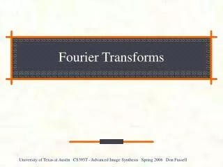
Y y Z P(Y,Z) r dydz R Y x X z Z April 26,29 Fourier methods in diffraction theory 11.3.4 Fourier methods in diffraction theory Fraunhofer diffraction: Aperture function: The field distribution over the aperture: A(y, z) = A0(y, z) exp[if (y, z)] • Each image point corresponds to a spatial frequency. • The field distribution of the Fraunhofer diffraction pattern is the Fourier transform of the aperture function:
A(z) E(kZ) z kZ b/2 -b/2 2p/b The single slit: Rectangular aperture: Fraunhofer-: The light interferes destructively here. Fourier-: The source has no spatial frequency here. The double slit (with finite width): f(z) h(z) g(z) = z z z b/2 -b/2 a/2 -a/2 a/2 -a/2 F(kZ) H(kZ) G(kZ) × = kZ kZ kZ
F(kZ) kZ Three slits: |F(kZ)|2 F(kZ) f(z) kZ kZ z 0 a -a Apodization: Removing the secondary maximum of a diffraction pattern. • Rectangular aperture sinc function secondary maxima. • Circular aperture Bessel function (Airy pattern) secondary maxima. • Gaussian aperture Gaussian function no secondary maxima. f(z) z
Array theorem: The Fraunhofer diffraction pattern from an array of identical apertures = The Fourier transform of an individual aperture × The Fourier transform of a set of point sources arrayed in the same manner. Convolution theorem z z = y y y Example: The double slit (with finite width).
Read: Ch11: 3 Homework: Ch11: 37,38,40 Due: May 3
May 1 Spectra and correlation 11.3.4 Spectra and correlation Considering a laser pulse described by E(t) = f (t). The temporal radiant flux is The total energy is Parseval(1755-1836, French mathematician)’s formula: If F(w) =F{f(t)}, then |F(w)|2 is the power spectrum. Unitarity of Fourier transform
f (t) t Application: Lorentzian profile: g w w0
Nature line width:The frequency bandwidth caused by the finite lifetime of the excited states. Line broadening mechanisms: • Natural broadening: Governed by the uncertainty principle. Lorentzian profile. • Doppler broadening: The light emitted will be red or blue shifted depending on the velocity of the emitting atoms relative to the observer. Gaussian profile. • Pressure broadening: The collision with other atoms interrupts the emission process. Lorentzian profile. Autocorrelation: The autocorrelation of f (t) is Wiener-Khintchine theorem: Determining the spectrum by autocorrelation: Symbol: cff (t) = f (t)f (t). Prove: Let h(t) = f *(-t), then
Cross Correlation: The cross correlation of f (t) and h(t) is Symbol: cfh(t) = f(t)h(t). For real functions, Properties (please prove them): 1) f (t)h(t) = f *(-t)h(t). Can be treated as the definition of cross correlation. 2) If f is an even function, then f (t)h(t) = f (t)h(t). 3) Cross-correlation theorem: F{f(t)h(t)} = F{f (t)}* ·F{h(t)} Applications of cross correlation: Optical pattern recognition Optical character recognition Rotational fitting in laser spectroscopy
Read: Ch11: 3 Homework: Ch11: 39,49,50 Due: May 8
All the world’s a stage, and all the men and women merely players. William Shakespeare