Download
1 / 49

E N D
Motivations Suppose you want to find all the files under a directory that contains a particular word. How do you solve this problem? There are several ways to solve this problem. An intuitive solution is to use recursion by searching the files in the subdirectories recursively.
Motivations The H-tree is used in VLSI design as a clock distribution network for routing timing signals to all parts of a chip with equal propagation delays. How do you write a program to display the H-tree? A good approach to solve this problem is to use recursion.
Objectives • To describe what a recursive function is and the benefits of using recursion (§15.1). • To develop recursive functions for recursive mathematical functions (§§15.2–15.3). • To explain how recursive function calls are handled in a call stack (§§15.2–15.3). • To use a helper function to derive a recursive function (§15.5). • To solve selection sort using recursion (§15.5.1). • To solve binary search using recursion (§15.5.2). • To get the directory size using recursion (§15.6). • To solve the Towers of Hanoi problem using recursion (§15.7). • To draw fractals using recursion (§15.8). • To solve the Eight Queens problem using recursion (§15.9). • To discover the relationship and difference between recursion and iteration (§15.10). • To know tail-recursive functions and why they are desirable (§15.11).
Computing Factorial factorial(0) = 1; factorial(n) = n*factorial(n-1); n! = n * (n-1)! ComputeFactorial
animation Computing Factorial factorial(0) = 1; factorial(n) = n*factorial(n-1); factorial(3)
animation Computing Factorial factorial(0) = 1; factorial(n) = n*factorial(n-1); factorial(3) = 3 * factorial(2)
animation Computing Factorial factorial(0) = 1; factorial(n) = n*factorial(n-1); factorial(3) = 3 * factorial(2) = 3 * (2 * factorial(1))
animation Computing Factorial factorial(0) = 1; factorial(n) = n*factorial(n-1); factorial(3) = 3 * factorial(2) = 3 * (2 * factorial(1)) = 3 * ( 2 * (1 * factorial(0)))
animation Computing Factorial factorial(0) = 1; factorial(n) = n*factorial(n-1); factorial(3) = 3 * factorial(2) = 3 * (2 * factorial(1)) = 3 * ( 2 * (1 * factorial(0))) = 3 * ( 2 * ( 1 * 1)))
animation Computing Factorial factorial(0) = 1; factorial(n) = n*factorial(n-1); factorial(3) = 3 * factorial(2) = 3 * (2 * factorial(1)) = 3 * ( 2 * (1 * factorial(0))) = 3 * ( 2 * ( 1 * 1))) = 3 * ( 2 * 1)
animation Computing Factorial factorial(0) = 1; factorial(n) = n*factorial(n-1); factorial(3) = 3 * factorial(2) = 3 * (2 * factorial(1)) = 3 * ( 2 * (1 * factorial(0))) = 3 * ( 2 * ( 1 * 1))) = 3 * ( 2 * 1) = 3 * 2
animation Computing Factorial factorial(0) = 1; factorial(n) = n*factorial(n-1); factorial(4) = 4 * factorial(3) = 4 * 3 * factorial(2) = 4 * 3 * (2 * factorial(1)) = 4 * 3 * ( 2 * (1 * factorial(0))) = 4 * 3 * ( 2 * ( 1 * 1))) = 4 * 3 * ( 2 * 1) = 4 * 3 * 2 = 4 * 6 = 24
animation Trace Recursive factorial Executes factorial(4)
animation Trace Recursive factorial Executes factorial(3)
animation Trace Recursive factorial Executes factorial(2)
animation Trace Recursive factorial Executes factorial(1)
animation Trace Recursive factorial Executes factorial(0)
animation Trace Recursive factorial returns 1
animation Trace Recursive factorial returns factorial(0)
animation Trace Recursive factorial returns factorial(1)
animation Trace Recursive factorial returns factorial(2)
animation Trace Recursive factorial returns factorial(3)
animation Trace Recursive factorial returns factorial(4)
Other Examples f(0) = 0; f(n) = n + f(n-1);
Fibonacci Numbers Fibonacci series: 0 1 1 2 3 5 8 13 21 34 55 89… indices: 0 1 2 3 4 5 6 7 8 9 10 11 fib(0) = 0; fib(1) = 1; fib(index) = fib(index -1) + fib(index -2); index >=2 fib(3) = fib(2) + fib(1) = (fib(1) + fib(0)) + fib(1) = (1 + 0) +fib(1) = 1 + fib(1) = 1 + 1 = 2 ComputeFibonacci
Characteristics of Recursion All recursive methods have the following characteristics: • One or more base cases (the simplest case) are used to stop recursion. • Every recursive call reduces the original problem, bringing it increasingly closer to a base case until it becomes that case. In general, to solve a problem using recursion, you break it into subproblems. If a subproblem resembles the original problem, you can apply the same approach to solve the subproblem recursively. This subproblem is almost the same as the original problem in nature with a smaller size.
Problem Solving Using Recursion Let us consider a simple problem of printing a message for n times. You can break the problem into two subproblems: one is to print the message one time and the other is to print the message for n-1 times. The second problem is the same as the original problem with a smaller size. The base case for the problem is n==0. You can solve this problem using recursion as follows: def nPrintln(message, times): if times >= 1: print(message) nPrintln(message, times - 1) # The base case is times == 0
Think Recursively Many of the problems presented in the early chapters can be solved using recursion if you think recursively. For example, the palindrome problem in Listing 8.1 can be solved recursively as follows: def isPalindrome(s): if len(s) <= 1: # Base case return True elif s[0] != s[len(s) - 1]: # Base case return False else: return isPalindrome(s[1 : len(s) – 1])
Recursive Helper Methods The preceding recursive isPalindrome method is not efficient, because it creates a new string for every recursive call. To avoid creating new strings, use a helper method: def isPalindrome(s): return isPalindromeHelper(s, 0, len(s) - 1) def isPalindromeHelper(s, low, high): if high <= low: # Base case return True elif s[low] != s[high]: # Base case return False else: return isPalindromeHelper(s, low + 1, high - 1)
Recursive Selection Sort • Find the smallest number in the list and swaps it with the first number. • Ignore the first number and sort the remaining smaller list recursively. RecursiveSelectionSort
Recursive Binary Search • Case 1: If the key is less than the middle element, recursively search the key in the first half of the array. • Case 2: If the key is equal to the middle element, the search ends with a match. • Case 3: If the key is greater than the middle element, recursively search the key in the second half of the array. RecursiveBinarySearch
Recursive Implementation def recursiveBinarySearch(list, key): low = 0 high = len(list) - 1 return recursiveBinarySearchHelper(list, key, low, high) def recursiveBinarySearchHelper(list, key, low, high): if low > high: # The list has been exhausted without a match return -low - 1 mid = (low + high) // 2 if key < list[mid]: return recursiveBinarySearchHelper(list, key, low, mid - 1) elif key == list[mid]: return mid else: return recursiveBinarySearchHelper(list, key, mid + 1, high) def main(): list = [3, 5, 6, 8, 9, 12, 34, 36] print(recursiveBinarySearch(list, 3)) print(recursiveBinarySearch(list, 4)) main()
Directory Size The preceding examples can easily be solved without using recursion. This section presents a problem that is difficult to solve without using recursion. The problem is to find the size of a directory. The size of a directory is the sum of the sizes of all files in the directory. A directory may contain subdirectories. Suppose a directory contains files , , ..., , and subdirectories , , ..., , as shown below.
Directory Size The size of the directory can be defined recursively as follows: DirectorySize
Towers of Hanoi • There are n disks labeled 1, 2, 3, . . ., n, and three towers labeled A, B, and C. • No disk can be on top of a smaller disk at any time. • All the disks are initially placed on tower A. • Only one disk can be moved at a time, and it must be the top disk on the tower.
Solution to Towers of Hanoi The Towers of Hanoi problem can be decomposed into three subproblems.
Solution to Towers of Hanoi • Move the first n - 1 disks from A to C with the assistance of tower B. • Move disk n from A to B. • Move n - 1 disks from C to B with the assistance of tower A. TowersOfHanoi
Fractals? A fractal is a geometrical figure just like triangles, circles, and rectangles, but fractals can be divided into parts, each of which is a reduced-size copy of the whole. There are many interesting examples of fractals. This section introduces a simple fractal, called Sierpinski triangle, named after a famous Polish mathematician.
Sierpinski Triangle • It begins with an equilateral triangle, which is considered to be the Sierpinski fractal of order (or level) 0, as shown in Figure (a). • Connect the midpoints of the sides of the triangle of order 0 to create a Sierpinski triangle of order 1, as shown in Figure (b). • Leave the center triangle intact. Connect the midpoints of the sides of the three other triangles to create a Sierpinski of order 2, as shown in Figure (c). • You can repeat the same process recursively to create a Sierpinski triangle of order 3, 4, ..., and so on, as shown in Figure (d).
Sierpinski Triangle Solution SierpinskiTriangle
Eight Queens EightQueens
Recursion vs. Iteration Recursion is an alternative form of program control. It is essentially repetition without a loop. Recursion bears substantial overhead. Each time the program calls a method, the system must assign space for all of the method’s local variables and parameters. This can consume considerable memory and requires extra time to manage the additional space.
Advantages of Using Recursion Recursion is good for solving the problems that are inherently recursive.
Tail Recursion A recursive method is said to be tail recursive if there are no pending operations to be performed on return from a recursive call. Non-tail recursive ComputeFactorial Tail recursive ComputeFactorialTailRecursion