Download
1 / 36
360 likes | 456 Vues
Measurement and Data Evaluation Course. Module 14 - Soil Classification with KSSL and field lab data. Why is this topic important?. Proper taxonomic classification of soils often requires laboratory data whether it comes from the KSSL or your office lab

E N D
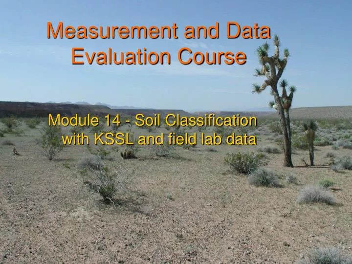
Measurement and Data Evaluation Course Module 14 - Soil Classification with KSSL and field lab data
Why is this topic important? • Proper taxonomic classification of soils often requires laboratory data whether it comes from the KSSL or your office lab • Knowing how to interpret measurements is critical to using data with Soil Taxonomy • The more you use laboratory data the better you will understand its value and also its limits as a tool for the soil survey
Objectives • Present examples of soil classification with KSSL and field laboratory data • Understand the limitations of lab data • Evaluate laboratory data to answer questions on taxonomic classification • Encourage the use of both KSSL and local lab data
Soil Classification with Laboratory DataGeneral Concepts • Soil Taxonomy has criteria tied to operational definitions such as PSC, Clay content, etc. • Significant Figures. – Classify pedons rigorously according to the precision required in Soil Taxonomy. • Rounding Conventions. – Perform any calculations on lab data before using standard rules to round to the significant digit used in the criteria. (e.g. wt. ave. 17.5 % = 18 %)
Soil Classification with Laboratory DataGeneral Concepts • Individual Values. - Convention is that lab data is reported one decimal beyond the dependable digit (in 30.4, the 0.4 is not certain). • Ratios. – Precision is dependent on precision of both the numerator and denominator values. • Ratios. – Precision is poorest when denominator value is low. Ratio of 1500 kPa water/Clay is not reliable when clay contents are < 5-8 %. • Units. – Use care in reading SSL datasets since many data are now reported in SI units. An example is centimoles per kilogram vs. milliequivalents per 100 g for data such as CEC; cmol/kg are not the same as mmol/L for analytes such as Ca in water extracted from saturated paste. mmol/L not the same as mmhos/cm (old unit for EC).
Soil Classification with Laboratory DataGeneral Concepts • Users should examine data for: • Internal consistency (values “out of place”) • Lithologic continuity or discontinuity • Pedologic continuity or discontinuity • Graph data for visual comparisons • Plot major sand fraction on a clay-free base vs. depth to check for continuity • Plot clay content, OM content, EC, etc. with depth to detect patterns of pedogenesis
Soil Classification with Laboratory DataGeneral Concepts • Realize data limitations/problems • Older lab datasets may lack needed tests and archive samples don’t exist to run them now • Results inconclusive to answer your questions (e.g. values may straddle criteria limits) • Horizon samples gathered may not be adequate or reflect needed property data at critical depths (e.g. base saturation for Ultisols, see p.33 of Keys) • Pedons sampled may not be representative
Stages of Taxonomic Classification • Initial assumptions based on: • existing soil survey information • field observations • research/special studies • Data collection to support assumptions • Survey documentation (points, transects, traverses) • Soil sampling for laboratory tests (field, SSL, Univ., commercial) • Final classification based on: • Evaluating documentation and lab data
Case study on a soil series Sondoa is a benchmark soil (moderate extent-90K) for MLRA 27 that had never been sampled. Current taxonomic classification is: Fine-silty, mixed, superactive, calcareous, mesic Typic Torriorthents Type location for this saline-sodic soil has always been in native (unreclaimed) salt-desert shrub rangeland. Several components in Lovelock Area (NV602) are mapped as slightly saline phases which are irrigated and reclaimed of excess salts and sodium.
Case study on a soil series Decision was made to sample a pedon of Sondoa near the present type location (rangeland) to gather characterization data on the largest component in the MLRA and survey area of origin. Taxonomic classifications may differ in the rangeland vs. cropland. Irrigated cropland may be reclaimed of excess salts and sodium.
Sample Site for Sondoa pedon in Humboldt Sink near Lovelock, NV
Case study on a soil series • Sampled pedon of Sondoa classifies as: Fine-silty, mixed, superactive, mesic Typic Haplosalid • Final classification decisions are pending on Sondoa components • Likely that Sondoa components in cropland leached of excess salts will be correlated as reclaimed phases and classified Sondoa series if extent is small
Classification Exercise Determining mineralogy class with laboratory data Background info: • The control section depths are given • Chose either the mixed or isotic class • All five pedons are noncalcareous • Key to mineralogy classes is on page 303 of the Keys to Soil Taxonomy, 10th ed. and will also be displayed onscreen
Classification Exercise Procedure: 1.) Open Excel file: “Mineralogy_Exercise.xls” 2.) Click tab for your team’s pedon to see data 3.) Apply mineralogy class criteria and assign class to the horizons in the PSCS of the pedon 4.) Determine and document (why?) the overall mineralogy class for the pedon 5.) One member of team shares answers onscreen in Adobe Connect window
Classification Exercise Determine the mineralogy class of your team’s assigned pedon Team 1 – Redhome Team 2 – Vicee Team 3 – Witefels Team 4 – Sibelia Team 5 – Cagwin
Key to Mineralogy Classes (section E.) E. All other mineral soil layers or horizons, in the mineralogy control section, that have: 1. More than 40 percent (by weight) (70 percent by grain count) mica and stable mica pseudomorphs in the 0.02 to 0.25 mm fraction. Micaceous or 2. More than 25 percent (by weight) (45 percent by grain count) mica and stable mica pseudomorphs in the 0.02 to 0.25 mm fraction. Paramicaceous or 3. A total percent (by weight) iron oxide as Fe2O3 (percent Fe by dithionate citrate times 1.43) plus the percent (by weight) gibbsite of more than 10 in the fine-earth fraction. Parasesquic or 4. In more than one-half of the thickness, all of the following: a. No free carbonates; and b. NaF pH of 8.4 or more; and c. A ratio of 1500 kPa water to measured clay of 0.6 or more. Isotic or 5. More than 90 percent (by weight or grain count) silica minerals (quartz, chalcedony, or opal) and other resistant minerals in the 0.02 to 2.0 mm fraction. Siliceous or 6. All other properties. Mixed
Considerations in using Lab Data • Don’t mix observations with concepts. • Observe first and then build basic inferences • Don’t predetermine the inferences • Initial concepts on taxonomic criteria and their operational definitions can change or evolve (stay current for your local issues) • Horizon designations (observations and interpretations of genesis) DO NOT equal taxonomic classifications
Considerations in using Lab Data • Know the analyses involved in an observation or measurement. • Results differ with different methods • To compare data, know how they were determined • Lab procedures and Soil Taxonomy use operational definitions (i.e. methods described in SSIR No. 42) • Recognize that operational and conceptual definitions are not the same.
Considerations in using Lab Data • Learn the rules of thumb and equations for laboratory data. • See SSIR 42 (2004) and 45 (1995) • Some examples (chemical data): • Gypsum is rarely present if pH >8.2 • Check for gypsum if Ca in saturated paste extract is >20 mmol (+)/L(-1) and pH is <8.2 • Gypsum is ‘usually present’ if Ca and SO4 in saturated paste extract is >20 mmol (+)/L(-1) (Nelson,1982) • % base saturation sum of cations (CEC-8.2) differs from base saturation by ammonium acetate (CEC-7.0) by a factor of about 0.7 (range is ~ 0.64-0.75)
Considerations in using Lab Data • Learn the rules of thumb and equations for laboratory data. • More examples (carbon): • Organic carbon (OC) is no longer directly measured by the SSL so total carbon (TC) by dry combustion must be used • In noncalcareous soils: %OC = %TC • %OC = %TC - (<2mm CaCO3* 0.12) is used in calcareous soils • %OM = %OC * 1.724 (Van Bemmelen factor) • C:N ratio relates to fertility and OM decomposition. C:N ratios of surface horizons (e.g. mollic epipedons) usually about 10 to 12; forest soils are higher.
Why collect local lab data? • Cons • Takes time, effort, & equipment • Management may not be supportive • Results can be confusing or conflicting • Uncertainty/anxiety • Pros • Faster results than analytical laboratories • Ownership of data • Learning experience • You gain confidence
Local tests to supplement SSL data • Chemical. • 1:1 H2O pH, NaF pH (an Isotic criterion) • KOH-Al (indicator only for Andic/Spodic) • Alpha,alpha-dipyridyl (for Fe reduction) • CEC, ECEC, % Base saturation (Hach kit) • % CaCO3 equivalent (e.g. Holmgren), % CO3-clay • Effervescence class (“free carbonates”) • % Gypsum and Equivalent gypsum content (EGC) • Electrical conductivity (saturated paste) • Sodium adsorption ratio (SAR) • Sodium-pyrophosphate color (organic materials)
Local tests to supplement SSL data • Physical. • PSDA • sand fractions • volcanic glass content • Ksat • water content • bulk density (by core & compliant cavity) • COLE • Atterberg limits (LL, PL, PI)
Local tests to supplement SSL data • Other technologies. • Electromagnetic induction (EMI) • Ground penetrating radar (GPR) • On-site data loggers (soil climate studies) • Wells, piezometers, Iris tubes, volt meters for redox potential (Eh), etc. -- (aquic conditions studies)
EMI data from salinity transect Minimum EC for Salic horizon
Summary • Laboratory data is part of the technology toolkit you need for taxonomic classification. • Criteria used in any taxonomic soil classification are mixtures of field-observations and laboratory (SSL and field) measurements. • Consider using local lab tests and the technology presented in this course to gather some of the data that you need.