Download
1 / 26
260 likes | 399 Vues
David Mould University of Saskatchewan Computational Aesthetics in Graphics, Visualization, and Imaging (2007). Stipple Placement using Distance in a Weighted Graph. OUTLINE. Stippling ─ a process whereby an image is constructed from a large number of small dots.

E N D
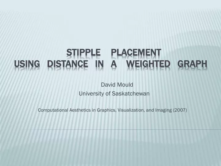
David Mould University of Saskatchewan Computational Aesthetics in Graphics, Visualization, and Imaging (2007) Stipple Placement using Distance in a Weighted Graph
Stippling ─ a process whereby an image is constructed from a large number of small dots. 1. Introduction
But Placing stipples by hand is a time-consuming process, and handmade stipple drawings contain fewer stipples than modern computer generated stipple images. • In computer graphics, stippling has been applied to the problem of halftoning. 1. Introduction
What is halftoning? • approximating a continuous-tone image with low color resolution but high spatial resolution (large numbers of dots). • Because having these property , halftoning couble be apply to printer technology • Three examples of color halftoning with CMYK separations. **in this paper just discuss color resolution in black and white 1. Introduction
Weighted Voronoi stippling .(Adrian Secord…..2002 NPAR) • provides a benchmark for high-quality stipple halftoning. WVS moves Voronoi centres to the centre of mass of the regions, where local density s given by darkness or some other measure of importance. • Recursive Wang tiles for real-time blue noise.(KOPF J., COHEN-OR D., DEUSSEN O.,LISCHINSKI D.....SIGGRAPH 2006) • speed up the stippling process, and have provided the ability to generate millions of stipple points per second. However, while these results can be used for halftoning, they do not attempt to treat sharp features. Previous Work
Human artists use stipples not only for tone reproduction,but also to illustrate features, including edge emphasis and texture indication. • In this paper they consider both darkness and gradient magnitude , so that to emphasize image feature ex: edge or some regions are dark in image. 2. Site Placement
Site Placement • This paper propose method operates by computing a least-cost path planningoperation through a weighted graph representation of the image, and progressively placing sitesof distance zero whenever the length of the shortest path exceeds a threshold. • Compute a least cost path using variant Dijkstra’s Algorithm. • Then placing sites by Progressive Algorithm. 2. Site Placement
Graph : construct a graph from an input image: a regular eight-connected lattice with one node per input image pixel. • Importance is computed for each node as αd +βg, where d is the darkness (1-intensity) and g is the gradient magnitude; α and β are normalizing factors, where we had α = 1/ d and β = 1/ g – that is, the inverses of the respective values summed over the entire image. • Edge weights are the average importances of the pixels on either end of the edge. 2. Site Placement
Dijkstra’s algorithm computes shortest distances from a source point to the other nodes in the graph. • Assume each node N has an estimated distance to the source , written E(N), and an actual distance, written A(N). • prepare a priority queue to store a set of “frontier” nodes: nodes with unknown actual distance but which lie adjacent to nodes with known actual distances. (* The priority queue is ordered by increasing estimated distance [min heap]) 2.1 Dijkstra’s Algorithm
Algorithm • Initially the frontier contains only the source node, at estimated distance zero and the graph is initialized with all nodes’ estimated distances set to infinity. • The top node, say T, is removed from the frontier, and its actual distance set to its estimated distance. • For each node Ni adjacent to T, a new estimate is computed Enew(Ni) as A(T) plus the cost of the edge linking Ni and T; those nodes whose old estimate exceeds Enew have their estimate replaced by the new estimate and are added to the frontier. • Goto (2) until when the frontier is empty, at which point all nodes in the graph have known distance values. *T is the top node in the frontier set. 2.1 Dijkstra’s Algorithm
Time Complexity To find the distances to n nodes, Dijkstra’s algorithm makes O(n) removal operations. Maintaining the heap has a cost of O(logm) per interaction , where m is the number of nodes in the frontier ; thus, the overall cost is O(nlogm). Typically, m << n ; that is, only a small fraction of the graph is in the heap at any one time . 2.1 Dijkstra’s Algorithm
Here propose a fast non-iterative algorithm for placing stipples. Site are placed progressively, building up a stippled region and adding new stipples at its fringe. 2.2. Progressive Site Placement
Algorithm • An initial seed(site) is placed at some location in the image. • use Dijkstra’s algorithm to expand a region around the seed(site). • check the path cost for a newly expanded node if exceeds a threshold the expansion step triggers the addition of a new stipple. (The new stipple location is the frontier node with highest gradient magnitude), and set new site N node’s E(N)=0 Goto(2) to expand new site region. else continue expansion original site region. until no part of the graph remains to be expanded, the progressive algorithm. * The new stipple location is the node with highest gradient magnitude since we want to place stipples preferentially on image edges. 2.2. Progressive Site Placement
A naive approach to search highest gradient magnitude node would require linear search of the entire frontier, But here we implement a second heap, ordered by gradient magnitude(Max Heap). Although requires a little extra memory, it makes the extraction process quite fast. • One feature of this algorithm is that the least-cost path between any two stipples is at minimum the chosen threshold. This property arises directly from the use of the frontier to place sites. At the time a new stipple is placed (triggered by the expansion of a node whose cost exceeds the threshold) all nodes on the frontier are at least the threshold distance away from the nearest stipple. • Distributions with a minimum separation between point are often identified as “blue noise”. 2.2. Progressive Site Placement
We are not restricted to faithfully matching the tones in an input image, however, and can instead construct an importance image that gives higher weight to areas such as edges. • In real images, especially photographic images, edges are common and the ability to express both intensity and edge information is invaluable. 3. Results
Left(5600):lowcontrast. Image edges, including details such as the whiskers and the fur direction in the ears, have been preserved. Right(9000):The prevalence of high-frequency detail, including wrinkles and facial hair, make this a challenging subject; despite the larger number of stipple,the features are not expressed clearly. 3. Results
Different stipple counts 3. Results
low stipple counts Lena(Left: WVS of gradient magnitude;Right: progressive stippling.) 3. Results
The times depend mainly on the resolution of the underlying graph, although there is a weak dependence on stipple count as well (since larger numbers of stipples tend to require larger heaps). 3. Results P4 -3.2G , 1GB , image resolution: 512 x 512
Mosaics and stipples have a close relationship: the same primitive distribution problems are seen in each. However, while stipples should be placed on image edges, mosaic tile centres should be placed away from edges. • Mosaics differ from stipples also in that beyond the problem of tile distribution, mosaics have the additional problems of tile shape and orientation. • we want to place new tiles at the lowest gradient location on the frontier, rather than the highest. • now care about the size of regions, rather than (strictly) the separation between tile centres. 4. Mosaic Construction
This latter point can be achieved by a straightforward conceptual modification of the algorithm: rather than placing a new centre when the path length exceeds a threshold, we place a new centre when the region size of the most recently placed tile exceeds a threshold. • we grow a single region at a time until it attains the desired size; as a new region grows, it is forbidden from growing into nodes already claimed by previously placed tiles. • this process often possess defects (such as holes), and we compute final tile shapes from a second pass of the distance calculation, starting from all tile centres simultaneously, labeling each node with its nearest tile centre. 4. Mosaic Construction
This Paper have described a novel stippling algorithm arising from progressive distance calculation over a graph representation of an input image. The method can capture both edge and darkness information, and is better suited to depicting sharp features than are previously proposed methods. • The output stippled images have blue-noise-like characteristics where features are absent, but are also able to show sharp features such as edges. • Our output is free of the distracting “chain” artifacts Voronoi packings are prone to. 5.Conclusions
Investigate methods for generating a more coherent depiction of high-frequency texture structure. • Would like to further explore and refine the application of this algorithm to irregular mosaics. • To incorporate stipple size changes into our framework. future work