Basic Concepts of Costs

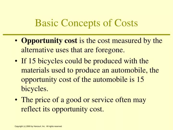
1. Basic Concepts of Costs • Opportunity cost is the cost measured by the alternative uses that are foregone. • If 15 bicycles could be produced with the materials used to produce an automobile, the opportunity cost of the automobile is 15 bicycles. • The price of a good or service often may reflect its opportunity cost.

2. Basic Concepts of Costs • Accounting cost is the concept that goods or services cost what was paid for them. • Economic cost is the amount required to keep a resource in its present use; the amount that it would be worth in its next best alternative use.

3. Labor Costs • Like accountants, economists regard the payments to labor as an explicit cost. • Labor services (worker-hours) are purchased at an hourly wage rate (w): The cost of hiring one worker for one hour.

4. Capital Costs • Accountants calculate capital costs by applying a depreciation rule. Economists view this as a sunk cost. • A sunk cost is an expenditure that once made cannot be recovered. • Economists consider the cost to be the amount someone else would pay for its use.- the rental rate (v).

5. Economic Profits and Cost Minimization • Economic profit ()

6. Cost-Minimizing Input Choice • Assume, for purposes of this chapter, that the firm has decided to produce a particular output level (say, q1). • The firm’s total revenues are P·q1. • How the firm might choose to produce this level of output at minimal costs is the subject of this chapter.

7. Cost-Minimizing Input Choice • Cost minimization requires that the marginal rate of technical substitution (RTS) of L for K equals the ratio of the inputs’ costs, w/v:

8. Graphic Presentation • The isoquant q1 shows all combinations of K and L that are required to produce q1. • The slope of total costs, TC = wL + vK, is -w/v. • Lines of equal cost will have the same slope so they will be parallel. • Three equal total costs lines, labeled TC1, TC2, and TC3 are shown in Figure 6.1.

9. FIGURE 6.1: Minimizing the Costs of Producing q1 Capital per week TC1 TC2 TC3 K* q1 0 Labor per week L*

10. Graphic Presentation • The minimum total cost of producing q1 is TC1 (since it is closest to the origin). • The cost-minimizing input combination is L*, K* which occurs where the total cost curve is tangent to the isoquant. • At the point of tangency, the rate at which the firm can technically substitute L for K (the RTS) equals the market rate (w/v).

11. An Alternative Interpretation • From Chapter 5 • Cost minimization requires • or, rearranging

12. The Firm’s Expansion Path • A similar analysis could be performed for any output level (q). • If input costs (w and v) remain constant, various cost-minimizing choices can be traces out as shown in Figure 6.2. • For example, output level q1 is produced using K1, L1, and other cost-minimizing points are shown by the tangency between the total cost lines and the isoquants.

13. The Firm’s Expansion Path • The firm’s expansion path is the set of cost-minimizing input combinations a firm will choose to produce various levels of output (when the prices of inputs are held constant). • Although in Figure 6.2, the expansion path is a straight line, that is not necessarily the case.

14. FIGURE 6.2: Firm’s Expansion Path Capital per week TC1 TC3 TC2 Expansion path q3 K1 q2 q1 Labor per week 0 L1

15. Cost Curves • A firm’s expansion path shows how minimum-cost input use increases when the level of output expands. • With this it is possible to develop the relationship between output levels and total input costs. • These cost curves are fundamental to the theory of supply.

16. Cost Curves • Figure 6.3 shows four possible shapes for cost curves. • In Panel a, output and required input use is proportional which means doubling of output requires doubling of inputs. This is the case when the production function exhibits constant returns to scale.

17. Cost Curves • Panels b and c reflect the cases of decreasing and increasing returns to scale, respectively. • With decreasing returns to scale the cost curve is convex, while the it is concave with increasing returns to scale. • Decreasing returns to scale indicate considerable cost advantages from large scale operations.

18. Cost Curves • Panel d reflects the case where there are increasing returns to scale followed by decreasing returns to scale. • This might arise because internal co-ordination and control by managers is initially underutilized, but becomes more difficult at high levels of output. • This suggests an optimal scale of output.

19. FIGURE 6.3: Possible Shapes of the Total Cost Curve TC Total cost Total cost TC 0 Quantity per week 0 Quantity per week (a) Constant Returns to Scale (b) Decreasing Returns to Scale TC Total cost Total cost TC 0 Quantity per week 0 Quantity per week (c) Increasing Returns to Scale (d) Optimal Scale

20. Average Costs • Average cost is total cost divided by output; a common measure of cost per unit. • If the total cost of producing 25 units is $100, the average cost would be

21. Marginal Cost • The additional cost of producing one more unit of output is marginal cost. • If the cost of producing 24 units is $98 and the cost of producing 25 units is $100, the marginal cost of the 25th unit is $2.

22. FIGURE 6.4: Average and Marginal Cost Curves AC, MC AC, MC MC AC AC, MC 0 Quantity per week 0 Quantity per week (a) Constant Returns to Scale (b) Decreasing Returns to Scale AC, MC AC AC, MC MC AC MC Quantity per week 0 q* Quantity per week 0 (c) Increasing Returns to Scale (d) Optimal Scale

23. Average Cost Curves • If a firm produces only one unit of output, marginal cost would be the same as average cost • Thus, the graph of the average cost curve begins at the point where the marginal cost curve intersects the vertical axis.

24. Average Cost Curves • For the constant returns to scale case, marginal cost never varies from its initial level, so average cost must stay the same as well. • Thus, the average cost curve are the same horizontal line as shown in Panel a of Figure 6.4.

25. Average Cost Curves • The U-shaped marginal cost curve shown in Panel d of Figure 6.4 reflects decreasing marginal costs at low levels of output and increasing marginal costs at high levels of output. • As long as marginal cost is below average cost, the marginal will pull down the average.

26. Average Cost Curves • When marginal costs are above average cost, the marginal pulls up the average. • Thus, the average cost curve must intersect the marginal cost curve at the minimum average cost; q* in Panel d of Figure 6.4. • Since q* represents the lowest average cost, it represents an “optimal scale” of production for the firm.

27. APPLICATION 6.2: Findings on Long-Run Costs • Entries in Table 1 represent long-run average cost estimates for different size firms as a percentage of the minimal average-cost firm in the industry. • These estimates, except for trucking, suggest lower average cost for medium and large firms. • Figure 1 shows the average cost firm suggested by the data.

28. FIGURE 1: Long-Run Average Cost Curve Found in Many Empirical Studies Average cost AC Quantity per period 0 q*

29. TABLE 1: Long-Run Average-Cost Estimates

30. APPLICATION 6.3: Airlines’ Costs • Costs for airlines have been of interest to economists because of recent changes such as deregulation, bankruptcy, and mergers. • Two general findings: • Costs seem to differ substantially among U.S. firms. • Costs for U.S. airlines appear to be significantly lower than for airlines in other countries.

31. Reasons for Differences among U.S. Firms • Airlines that fly longer average distances or operate a greater number of flights over a given network tend to have lower costs. • Firms can spread the fixed costs associated with terminals, maintenance facilities, and reservation systems over a larger output volume.

32. International Airline Regulation and Costs • Many foreign carriers’ have not adopted the “hub and spoke” system which appears to be more efficient. • Foreign firms are subject to more regulation. • This situation appears to be changing. For example, Australia ended rigid controls and costs fell by 15 to 20 percent.

33. Distinction between the Short Run and the Long Run • The short run is the period of time in which a firm must consider some inputs to be absolutely fixed in making its decisions. • The long run is the period of time in which a firm may consider all of its inputs to be variable in making its decisions.

34. Short-Run Total Costs • Total cost for the firm is TC = vK + wL • The short-run analysis is denoted by STC = vK1 + wL. • The term vK1 is called (short-run) fixed costs; costs associated with inputs that are fixed in the short run.

35. Short-Run Total Costs • The term wL is referred to as (short-run) variable costs; costs associated with inputs that can be varied in the short run. • Using the terms SFC for short-run fixed costs and SVC for short-run variable costs, the firms short-run costs are given by STC = SFC + SVC.

36. FIGURE 6.5: Fixed and Variable Costs in the Short Run Fixed costs Variable costs SVC SFC 0 Quantity per week 0 q’ Quantity per week (a) Short-Run Fixed Cost Curve (b) Short-Run Variable Cost Curve

37. Short-Run Variable Cost Curve • Beyond some output level, say q’, however, the marginal product of labor will eventually decline causing the costs of production to rise rapidly. • This implies that the short-run variable cost curve (SVC) will then be convex beyond q’.

38. Short-Run Total Cost Curve • The short-run total cost curve is the summation of the short-run fixed cost curve and the short-run variable cost curve. • This curve, which is shown in Figure 6.6, intersects the vertical axis at SFC and has the shape of the SVC curve.

39. FIGURE 6.6: Short-Run Total Cost Curve STC Total costs SFC Quantity per week 0

40. Per-Unit Short-Run Cost Curves

41. Per-Unit Short-Run Cost Curves • Having capital fixed in the short run yields a total cost curve that has both concave and convex sections, the resulting short-run average and marginal cost relationships will also be U-shaped. • These two curves are shown in Figure 6.8. • When SMC < SAC, average cost is falling, but when SMC > SAC average cost increase.

42. FIGURE 6.8: Per-Unit Short-Run Cost Curves Unit cost SMC SAC Quantity per week 0

43. Relationship between Short-Run and Long-Run per-Unit Cost Curves • Figure 6.9 shows all cost relationships for a firm that has U-shaped long-run average and marginal cost curves. • At output level q* long-run average costs are minimized and MC = AC. • Associated with q* is a certain level of capital, K*.

44. FIGURE 6.9: Short-Run and Long-Run Average and Marginal Cost Curves at Optimal Output Level AC, MC MC AC SMC SAC 0 q* Quantity per week

45. Relationship between Short-Run and Long-Run per-Unit Cost Curves • In the short-run, when the firm using K* units of capital produces q*, short-run and long-run total costs are equal. • In addition, as shown in Figure 6.9 AC = MC = SAC(K*) = SMC(K*). • For output above q* short-run costs are higher than long-run costs. The higher per-unit costs reflect the facts that K is fixed.

46. Shifts in Cost Curves • Any change in economic conditions that affects the expansion path will also affect the shape and position of the firm’s cost curves. • Three sources of such change are: • change in input prices • technological innovations, and • economies of scope.