Download
1 / 49
490 likes | 496 Vues
This article explores clustering techniques for grouping similar objects and labeling them. It discusses different types of clustering algorithms, such as flat and hierarchical clustering, and the distinction between hard and soft assignment. The advantages and limitations of each algorithm are summarized.

E N D
Clustering Techniques Berlin Chen 2005 References: • Introduction to Machine Learning , Chapter 7 • Modern Information Retrieval, Chapters 5, 7 • Foundations of Statistical Natural Language Processing, Chapter 14 • "A Gentle Tutorial of the EM Algorithm and its Application to Parameter Estimation for Gaussian Mixture and Hidden Markov Models," Jeff A. Bilmes, U.C. Berkeley TR-97-021
Clustering • Place similar objects in the same group and assign dissimilar objects to different groups • Word clustering • Neighbor overlap: words occur with the similar left and right neighbors (such as in and on) • Document clustering • Documents with the similar topics or concepts are put together • But clustering cannot give a comprehensive description of the object • How to label objects shown on the visual display • Regarded as a kind of semiparametric learning approach • Allow a mixture of distributions to be used for estimating the input samples (a parametric model for each group of samples)
Clustering vs. Classification • Classification is supervised and requires a set of labeled training instances for each group (class) • Clustering is unsupervised and learns without a teacher to provide the labeling information of the training data set • Also called automatic or unsupervised classification
Types of Clustering Algorithms • Two types of structures produced by clustering algorithms • Flat or non-hierarchical clustering • Hierarchical clustering • Flat clustering • Simply consisting of a certain number of clusters and the relation between clusters is often undetermined • Measure: construction error minimization or probabilistic optimization • Hierarchical clustering • A hierarchy with usual interpretation that each node stands for a subclass of its mother’s node • The leaves of the tree are the single objects • Each node represents the cluster that contains all the objects of its descendants • Measure: similarities of instances
Hard Assignment vs. Soft Assignment • Another important distinction between clustering algorithms is whether they perform soft or hard assignment • Hard Assignment • Each object is assigned to one and only one cluster • Soft Assignment (probabilistic approach) • Each object may be assigned to multiple clusters • An object has a probability distribution overclusters where is the probability that is a member of • Is somewhat more appropriate in many tasks such as NLP, IR, …
Hard Assignment vs. Soft Assignment (cont.) • Hierarchical clustering usually adopts hard assignment • While in flat clustering both types of assignments are common
Summarized Attributes of Clustering Algorithms • Hierarchical Clustering • Preferable for detailed data analysis • Provide more information than flat clustering • No single best algorithm (each of the algorithms only optimal for some applications) • Less efficient than flat clustering (minimally have to compute n x n matrix of similarity coefficients)
Summarized Attributes of Clustering Algorithms (cont.) • Flat Clustering • Preferable if efficiency is a consideration or data sets are very large • K-means is the conceptually method and should probably be used on a new data because its results are often sufficient • K-means assumes a simple Euclidean representation space, and so cannot be used for many data sets, e.g., nominal data like colors (or samples with features of different scales) • The EM algorithm is the most choice. It can accommodate definition of clusters and allocation of objects based on complex probabilistic models • Its extensions can be used to handle topological/hierarchical orders of samples • Probabilistic Latent Semantic Analysis (PLSA), Topic Mixture Model (TMM), etc.
Hierarchical Clustering • Can be in either bottom-up or top-down manners • Bottom-up (agglomerative) • Start with individual objects and grouping the most similar ones • E.g., with the minimum distance apart • The procedure terminates when one cluster containing all objects has been formed • Top-down (divisive) • Start with all objects in a group and divide them into groups so as to maximize within-group similarity 凝集的 distance measures will be discussed later on 分裂的
Hierarchical Agglomerative Clustering (HAC) • A bottom-up approach • Assume a similarity measure for determining the similarity of two objects • Start with all objects in a separate cluster and then repeatedly joins the two clusters that have the most similarity until there is one only cluster survived • The history of merging/clustering forms a binary tree or hierarchy
HAC (cont.) • Algorithm Initialization (for tree leaves): Each object is a cluster cluster number merged as a new cluster The original two clusters are removed
Distance Metrics • Euclidian Distance (L2 norm) • Make sure that all attributes/dimensions have the same scale (or the same variance) • L1 Norm (City-block distance) • Cosine Similarity (transform to a distance by subtracting from 1) ranged between 0 and 1
Ci Cj Measures of Cluster Similarity • Especially for the bottom-up approaches • Single-link clustering • The similarity between two clusters is the similarity of the two closest objects in the clusters • Search over all pairs of objects that are from the two different clusters and select the pair with the greatest similarity • Elongated clusters are achieved cf. the minimal spanning tree greatest similarity
Ci Cj Measures of Cluster Similarity (cont.) • Complete-link clustering • The similarity between two clusters is the similarity of their two most dissimilar members • Sphere-shaped clusters are achieved • Preferable for most IR and NLP applications least similarity
Measures of Cluster Similarity (cont.) single link complete link
Measures of Cluster Similarity (cont.) • Group-average agglomerative clustering • A compromise between single-link and complete-link clustering • The similarity between two clusters is the average similarity between members • If the objects are represented as length-normalized vectors and the similarity measure is the cosine • There exists an fast algorithm for computing the average similarity length-normalized vectors
Measures of Cluster Similarity (cont.) • Group-average agglomerative clustering (cont.) • The average similarity SIM between vectors in a cluster cj is defined as • The sum of members in a cluster cj : • Express in terms of length-normalized vector =1
Measures of Cluster Similarity (cont.) • Group-average agglomerative clustering (cont.) -As merging two clusters ci and cj , the cluster sum vectors and are known in advance • The average similarity for their union will be
Example: Word Clustering • Words (objects) are described and clustered using a set of features and values • E.g., the left and right neighbors of tokens of words higher nodes: decreasing of similarity “be” has least similarity with the other 21 words !
Divisive Clustering • A top-down approach • Start with all objects in a single cluster • At each iteration, select the least coherent cluster and split it • Continue the iterations until a predefined criterion (e.g., the cluster number) is achieved • The history of clustering forms a binary tree or hierarchy
Divisive Clustering (cont.) • To select the least coherent cluster, the measures used in bottom-up clustering (e.g. HAC) can be used again here • Single link measure • Complete-link measure • Group-average measure • How to split a cluster • Also is a clustering task (finding two sub-clusters) • Any clustering algorithm can be used for the splitting operation, e.g., • Bottom-up (agglomerative) algorithms • Non-hierarchical clustering algorithms (e.g., K-means)
: Divisive Clustering (cont.) • Algorithm split the least coherent cluster Generate two new clusters and remove the original one
Non-hierarchical Clustering • Start out with a partition based on randomly selected seeds (one seed per cluster) and then refine the initial partition • In a multi-pass manner (recursion/iterations) • Problems associated with non-hierarchical clustering • When to stop • What is the right number of clusters • Algorithms introduced here • The K-means algorithm • The EM algorithm group average similarity, likelihood, mutual information k-1 → k → k+1 Hierarchical clustering also has to face this problem
The K-means Algorithm • Also called Linde-Buzo-Gray (LBG) in signal processing • A hard clustering algorithm • Define clusters by the center of mass of their members • The K-means algorithm also can be regarded as • A kind of vector quantization • Map from a continuous space (high resolution) to a discrete space (low resolution) • E.g. color quantization • 24 bits/pixel (16 million colors) → 8 bits/pixel (256 colors) • A compression rate of 3 Dim(xt)=24 → k=28
The K-means Algorithm (cont.) • and are unknown • depends on and this optimization problem can not be solved analytically label
The K-means Algorithm (cont.) • Initialization • A set of initial cluster centers is needed • Recursion • Assign each object to the cluster whose center is closest • Then, re-compute the center of each cluster as the centroid or mean (average) of its members • Using the medoid as the cluster center ? (a medoid is one of the objects in the cluster) These two steps are repeated until stabilizes
The K-means Algorithm (cont.) • Algorithm
The K-means Algorithm (cont.) • Example 1
The K-means Algorithm (cont.) • Example 2 government finance sports research name
The K-means Algorithm (cont.) • Choice of initial cluster centers (seeds) is important • Pick at random • Calculate the mean of all data and generate k initial centers by adding small random vector to the mean • Project data onto the principal component (first eigenvector), divide it range into k equal interval, and take the mean of data in each group as the initial center • Or use another method such as hierarchical clustering algorithm on a subset of the objects • E.g., buckshot algorithm uses the group-average agglomerative clustering to randomly sample of the data that has size square root of the complete set • Poor seeds will result in sub-optimal clustering
The K-means Algorithm (cont.) • How to break ties when in case there are several centers with the same distance from an object • Randomly assign the object to one of the candidate clusters • Or, perturb objects slightly • Applications of the K-means Algorithm • Clustering • Vector quantization • A preprocessing stage before classification or regression • Map from the original space to l-dimensional space/hypercube Nodes on the hypercube l=log2k (k clusters) A linear classifier
The K-means Algorithm (cont.) • E.g., the LBG algorithm • By Linde, Buzo, and Gray {12,12,12} {11,11,11} Global mean Cluster 1 mean Cluster 2mean {13,13,13} {14,14,14} M→2M at each iteration
The EM Algorithm • A soft version of the K-mean algorithm • Each object could be the member of multiple clusters • Clustering as estimating a mixture of (continuous) probability distributions A Mixture Gaussian HMM (or A Mixture of Gaussians) Continuous case: Likelihood function for data samples:
Maximum Likelihood Estimation • Hard Assignment State S1 P(B| S1)=2/4=0.5 P(W| S1)=2/4=0.5
Maximum Likelihood Estimation • Soft Assignment State S1 State S2 0.7 0.3 0.4 0.6 P(B| S1)=(0.7+0.9)/ (0.7+0.4+0.9+0.5) =1.6/2.5=0.64 P(B| S2)=(0.3+0.1)/ (0.3+0.6+0.1+0.5) =0.4/1.5=0.27 0.9 0.1 0.5 0.5 P(B| S2)=(0.6+0.5)/ (0.3+0.6+0.1+0.5) =0.11/1.5=0.73 P(B| S1)=(0.4+0.5)/ (0.7+0.4+0.9+0.5) =0.9/2.5=0.36
The EM Algorithm (cont.) • E–step (Expectation) • Derive the complete data likelihood function likelihood function the complete data likelihood function
The EM Algorithm (cont.) unknown known • E–step (Expectation) • Define the auxiliary function as the expectation of the log complete likelihood function LCMwith respect to thehidden/latent variableC conditioned on known data • Maximize the log likelihood function by maximizing the expectation of the log complete likelihood function • We have shown this property when deriving the HMM-based retrieval model
The EM Algorithm (cont.) • E–step (Expectation) • The auxiliary function ? See Next Slide
The EM Algorithm (cont.) • Note that
The EM Algorithm (cont.) • E–step (Expectation) • The auxiliary function can also be divided into two: auxiliary function for mixture weights auxiliary function for cluster distributions
The EM Algorithm (cont.) • M-step (Maximization) • Remember that • Maximize a function F with a constraintby applying Lagrange multiplier Constraint
The EM Algorithm (cont.) • M-step (Maximization) • Maximize auxiliary function for mixture weights (or priors for Gaussians)
The EM Algorithm (cont.) • M-step (Maximization) • Maximize auxiliary function for (multivariate) Gaussian Means and Variances constant
The EM Algorithm (cont.) • M-step (Maximization) • Maximize with respect to
The EM Algorithm (cont.) • M-step (Maximization) • Maximize with respect to
The EM Algorithm (cont.) • The initial cluster distributions can be estimated using the K-means algorithm • The procedure terminates when the likelihoodfunction is converged or maximum numberof iterations is reached