Download
1 / 27
270 likes | 351 Vues
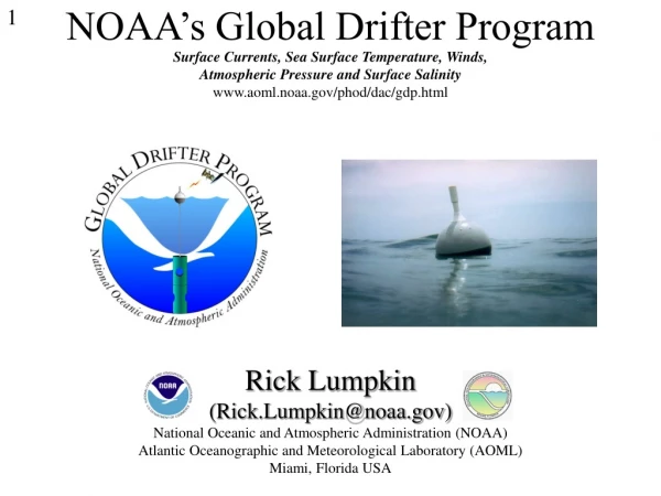
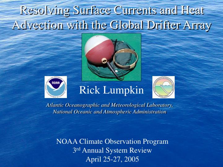
Resolving Surface Currents and Heat Advection with the Global Drifter Array. Rick Lumpkin. Atlantic Oceanographic and Meteorological Laboratory, National Oceanic and Atmospheric Administration. NOAA Climate Observation Program 3 rd Annual System Review April 25-27, 2005.

E N D
Resolving Surface Currents and Heat Advection with the Global Drifter Array Rick Lumpkin Atlantic Oceanographic and Meteorological Laboratory, National Oceanic and Atmospheric Administration NOAA Climate Observation Program 3rd Annual System Review April 25-27, 2005
75% of 1°1°bins! Time-mean currents
Mean heat advection SST gradient (°C per degree) Mean heat advection, upper 30m (W/m2)
Advection of SST anomalies W/m2 Anomalous heat advection, upper 30m (W/m2)
378 drogued Surface current anomalies
2. What we aren’t resolving (Drifters alone: any process happening in data gaps)
Evaluating the drifter array SST: GOOS evaluated by NOAA/NCDC SURFACE CURRENTS Accuracy: 2 cm/s Resolution: 600 km Number of measurements per month: 1 From Needler et al. 1999: Action plan for GOOS/GCOS and Sustained Observations for CLIVAR.
Include information from other measurements (altimetry, winds)
170ºE-130ºW, 10ºS-10ºN OSCAR Pilot project for a NOAA/NESDIS Operational Surface Current Processing and Data Center (F. Bonjean, J. Gunn, G. Lagerloef, E. Johnson)
AVISO Altimetry product Collecte Localisation Satellites (CLS) Topex/Poseidon, Jason-1, ERS-1 and ERS-2 Aviso
U(t)=U + A u’(t) Absolute speed (m/s) Drifters+wind, altimetry altimeter (methodology of Niiler et al., 2003)
L pg Coriolis centrifugal H Cor pg centrifugal H L large Rossby number flow (centrifugal) (Coriolis) (Pressure gradient) If we ignore centrifugal (assume geostrophy), we: Underestimate Coriolis (underestimate v) Overestimate Coriolis (overestimate v)
1 0.5 0 Drifters: calibrating satellite SSV
Drifters: in-situ calibration to reduce global bias in satellite SSV R. Lumpkin and G. Goni, NOAA/AOML
Summary: Global Drifter Array • What we can resolve: • <U>, <SST>, <U>·<SST>, • U(x,t) where coverage is sufficient • mean eddy statistics • Drifter SST(x, t): cal/val of satellite products • <U>· SST’ • What we can’t resolve: • Anything in the “data holes” • U(x,t) at sufficient resolution for time series • of eddy fluxes • What we can do about this: • Plan ahead: anticipate gaps • Synthesize drifters, winds and altimetry for • operational surface currents • Drifter U(x,t) cal/val of satellite products Rick.Lumpkin@noaa.gov