Download
1 / 26
260 likes | 269 Vues
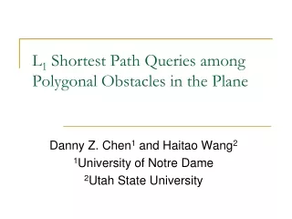
A Nearly Optimal Algorithm for Finding L 1 Shortest Paths among Polygonal Obstacles in the Plane. Danny Z. Chen and Haitao Wang University of Notre Dame Indiana, USA. Shortest paths among polygonal obstacles.

E N D
A Nearly Optimal Algorithm for Finding L1Shortest Paths among Polygonal Obstacles in the Plane Danny Z. Chen and Haitao Wang University of Notre Dame Indiana, USA
Shortest paths among polygonal obstacles • Input: A set of h polygonal obstacles with totally n vertices, and two points s and t • Output: A shortest path from s to t that avoids the obstacles t free space s obstacle
Our problem: the L1 version • L1 shortest path problem: Find a path from s to t with minimum L1 distance • The path can be arbitrarily polygonal • But the distance is measured by L1 metric vertical distance e horizontal distance The L1 distance of e = the horizontal distance + the vertical distance
Previous work (the first approach) • Construct a “path preserving graph” and then run Dijkstra’s algorithm on the graph • Key: The size of the graph should be as small as possible • O(nlog2n) time and O(nlogn) space, Clarkson, Kapoor, and Vaidya, 87’ • O(nlog1.5n) time and O(nlog1.5n) space, Clarkson, Kapoor, and Vaidya, 88’ • O(nlog1.5n) time and O(nlogn) space, Chen, Klenk, and Tu, 00’ • O(n+hlog1.5h) time and O(n+hlog1.5h) space, Inkulu and Kapoor, 09’ • a corridor structure
Previous work (the second approach) • Continuous Dijkstra paradigm s t
Continuous Dijkstra paradigm for L1 metric s The wavelets are of diamond shape
Previous work (cont.) • Continuous Dijkstra paradigm • O(nlogn) time and O(n) space, Mitchell 92’ • Lower bound: O(n+hlogh) time and O(n) space • Mitchell’s algorithm is worst case optimal
Our results O(T+n+hlogh) time and O(n) space T is the time for triangulating the free space T=O(n+hlog1+εh), Bar-Yehuda and Chazelle, 94’ t s obstacle
Our results (cont.) • O(T+n+hlogh) time and O(n) space • T is the time for triangulating the free space • T=O(n+hlog1+εh), Bar-Yehuda and Chazelle, 94’ • Build shortest path maps to answer L1 shortest path queries • Improvements on other problems • Shortest rectilinear path • Shortest L∞ path • Shortest path of c-orientations, for a given number c • Approximation algorithms for finding an Euclidean shortest path
Our approach • A combination of the corridor structure and the continuous Dijkstra paradigm (modifying Mitchell’s algorithm) • Use a corridor structure to somehow reduce the problem to the convex case where all obstacles are convex • Solve the convex case in O(n+hlogh) time and O(n) space
The convex case • Input: a set of h convex polygonal obstacles of totally n vertices • Output: a shortest path from s to t in the free space t s
The core of a convex obstacle • For any convex obstacle P, define its core to be the polygon by connecting the topmost, rightmost, bottommost, leftmost vertices of P The blue polygon is the core of the yellow obstacle
Why do we need the cores? • A critical observation: a shortest s-t path avoiding all cores the same L1 distance a shortest s-t path avoiding all input obstacles
Our algorithm for the convex case • Compute the core of each convex obstacle • Apply Mitchell’s algorithm on all cores to find a shortest path p from s to t avoiding all cores • Based on the path p, find a shortest path from s to t avoiding all input obstacles
An example t s
Our algorithm for the convex case • Compute the core of each convex obstacle • O(n) time • Apply Mitchell’s algorithm on all cores to find a shortest path p from s to t avoiding all cores • O(hlogh) time since all cores contains only O(h) vertices • Based on the path p, find a shortest path from s to t avoiding all input obstacles • O(n) time
Correctness of the algorithm • Ears of a convex obstacle c a e b f d
An example t s
Our algorithm for the general case • The obstacles are not convex t s obstacle
Our algorithm for the general case (cont.) • By using a corridor structure, partition the plane into a set P’ of O(h) convex obstacles of O(n) vertices, along with O(h) corridor paths contained in obstacles • P: the input obstacle set • A shortest path from s to t avoiding P is a shortest path avoiding P’ but possibly containing some corridor paths
An s-t path may contain some corridor paths a corridor path t s A standard technique used in the path preserving approach (also for the Euclidean case)
What’s new? • Modify the continuous Dijkstra paradigm on the convex obstacle set P’ and the corridor paths
Some algorithm details • Define the core of a convex obstacle in P’ differently • The endpoints of corridor paths are also considered as the core vertices • The total number of vertices in all cores of P’ is still O(h) • There are O(h) corridor paths an ordinary convex obstacle the obstacle contains a corridor path
Some algorithm details (cont.) • Whenever a wavelet encounters an endpoint a of a corridor path p, initiate a “pseudo-wavelet” at a • the event point: the other endpoint b of p • the even distance: the distance of the corridor path b s a There are O(h) such additional events for the endpoints of the corridor paths The overall running time of the modified Mithchell’s algorithm is still O(hlogh)
Conclusions • Using the cores to compute a shortest path • The combination of the corridor structure and the continuous Dijkstra paradigm