Download
1 / 65
780 likes | 1.42k Vues
Chapter 8 IDEAL-FLUID FLOW. In the preceding chapters most of the relations have been developed for one-dimensional flow, i.e., flow in which the average velocity at each cross section is used and variations across the section are neglected.

E N D
In the preceding chapters most of the relations have been developed for one-dimensional flow, i.e., flow in which the average velocity at each cross section is used and variations across the section are neglected. • Many design problems in fluid flow, however, require more exact knowledge of velocity and pressure distributions, such as in flow over curved boundaries along an airplane wing, through the passages of a pump or compressor, or over the crest of a dam. • An understanding of two- and three-dimensional flow of a nonviscous, incompressible fluid provides the student with a much broader approach to many real fluid-flow situations. There are also analogies that permit the same methods to apply to flow through porous media. • In this chapter the principles of irrotational flow of an ideal fluid are developed and applied to elementary flow cases. After the flow requirements are established, Euler's equation is derived and the velocity potential is defined.
8.1 REQUIREMENTS FOR IDEAL-FLUID FLOW • The Prandtl hypothesis states that for fluids of low viscosity the effects of viscosity are appreciable only in a narrow region surrounding the fluid boundaries. • For incompressible flow situations in which the boundary layer remains thin, ideal-fluid results may be applied to flow of a real fluid to a satisfactory degree of approximation. • An ideal fluid must satisfy the following requirements: • 1. The continuity equation div q = 0, or • 2. Newton's second law of motion at every point at every instant • 3. Neither penetration of fluid into, nor gaps between, fluid and boundary at any solid boundary
If, in addition to requirements 1, 2, and 3, the assumption of irrotational flow is made, the resulting fluid motion closely resembles real-fluid motion for fluids of low viscosity, outside boundary layers. • Using the above conditions, the application of Newton's second law to a fluid particle leads to the Euler equation, which, together with the assumption of irrotational flow, can be integrated to obtain the Bernoulli equation. The unknowns in a fluid-flow situation with given boundaries are velocity and pressure at every point. • Unfortunately, in most cases it is impossible to proceed directly to equations for velocity and pressure distribution from the boundary conditions.
8.2 EULER'S EQUATION OF MOTION • Euler's equation of motion along a streamline (one-dimensional) was developed in Sec. 3.5 by use of the momentum and continuity equations and Eq. (2.2.5). • In this section it is developed from Eq. (2.2.5) for the xyz-coordinate system in any orientation, with the assumption that gravity is the only body force acting. Since Euler's equation is based on a frictionless fluid, the vector equation (2.2.5) (2.2.5) • may be reorganized into the proper form. The unit vector j' is directed vertically upward in the coordinate direction h. • These are the direction cosines of h with respect to the xyz system of coordinates, and they may be written
Figure 8.1 Arbitrary orientation of xyz coordinate system
For example, ∂h/∂xis the change in h for unit change in x when y, z, and t are constant. In equation form, • The operation applied to the scalar h yields the gradient of h, as in Eq. (2.2.2). • Eq. (2.2.5) now becomes (8.2.1) • The component equations of Eq.(8.2.1) are (8.2.2)
u, v, w are velocity components in the x, y, z directions, respectively, at any point; du/dt is the x component of acceleration of the fluid particle at (x, y, z). • Since u is a function of x, y, z, and t and x, y, and z are coordinates of the moving fluid particle, they become functions of t;hence, • However, dx/dt, dy/dt, and dz/dt are the velocity components of the particle, so that ax, the x component of the particle acceleration, is
By treating dv/dt and dw/dt in a similar manner, the Euler equations in three dimensions for a frictionless fluid are (8.2.3) (8.2.4) (8.2.5) • The first three terms on the right-hand sides of the equations are convective-acceleration terms, depending upon changes of velocity with space. • The last term is local acceleration, depending upon velocity change with time at a point.
Natural Coordinates in Two-Dimensional Flow • Euler's equations in two dimensions are obtained from the general-component equations by setting w = 0 and ∂/∂z=0; thus (8.2.6) (8.2.7) • By taking particular directions for the x and y axes, they can be reduced to a form that makes them easier to understand. • The velocity component u is vs, and the component v is vn. As vnis zero at the point, Eq. (8.2.6) becomes (8.2.8) • Although vn is zero at the point (s, n), its rates of change with respect to s and t are not necessarily zero. Equation (8.2.7) becomes (8.2.9)
With r the radius of curvature of the streamline at s, from similar triangles (Fig. 8.2), • Substituting into Eq. (8.2.9) gives (8.2.10) • For steady flow of an incompressible fluid Eqs. (8.2.6) and (8.2.10) can be written (8.2.11) and (8.2.12) • Equation (8.2.11) can be integrated with respect to s to produce Eq. (3.6.1), with the constant of integration varying with n, that is, from one streamline to another. • Equation (8.2.12) shows how pressure head varies across streamlines. With vs and r known functions of n, Eq. (8.2.12) can be integrated.
Example 8.1 • A container of liquid is rotated with angular velocity ω about a vertical axis as a solid. Determine the variation of pressure in the liquid. Solution • n is the radial distance, measured inwardly, dn = -dr, and vs= ωr . Integrating Eq. (8.2.12) gives or • To evaluate the constant, if p = p0 when r = 0 and h = 0, • which shows that the pressure is hydrostatic along a vertical line and increases as the square of the radius. • Integration of Eq. (8.2.11) shows that the pressure is constant for a given h and vs, that is, along a streamline.
8.3 IRROTATIONAL FLOW; VELOCITY POTENTIAL • In this section it is shown that the assumption of irrotational flow leads to the existence of a velocity potential. By use of these relations and the assumption of a conservative body force, the Euler equations can be integrated. • The individual particles of a frictionless incompressible fluid initially at rest cannot be caused to rotate. This can be visualized by considering a small free body of fluid in the shape of a sphere. Surface forces act normal to its surface, since the fluid is frictionless, and therefore act through the center of the sphere. • Similarly, the body force acts at the mass center. Hence, no torque can be exerted on the sphere, and it remains without rotation. Likewise, once an ideal fluid has rotation, there is no way of altering it, as no torque can be exerted on an elementary sphere of the fluid.
An analytical expression for fluid rotation of a particle about an axis parallel to the z axis is developed. The rotation component may be defined as the average angular velocity of two infinitesimal linear elements that are mutually perpendicular to each other and to the axis of rotation. • The two line elements may conveniently be taken as x and y in Fig. 8.3, although any other two perpendicular elements in the plane through the point would yield the same result. The particle is at P(x, y), and it has velocity components u, v in the xy plane. The angular velocities of δx and δy are sought. • The angular velocity of δx is • and the angular velocity of δy is • if counterclockwise is positive. Hence, by definition, the rotation component ωz of a fluid particle at (x,y) is (8.3.1)
Similarly, the two other rotation components, ωxand ωy, about axes parallel to x and to y are (8.3.2) • The rotation vector ω is (8.3.3) • The vorticity vector, curl q = × q, is defined as twice the rotation vector. It is given by 2ω. • By assuming that the fluid has no rotation, i.e., it is irrotational, curl q = 0, or from Eqs. (8.3.1) and (8.3.2) (8.3.4) • These restrictions on the velocity must hold at every point (except special singular points or lines).
The first equation is the irrotational condition for two dimensional flow. It is the condition that the differential expression • is exact, say (8.3.5) • The minus sign is arbitrary; it is a convention that causes the value of φto decrease in the direction of the velocity. By comparing terms in Eq. (8.3.5), • In vector form, (8.3.6) • is equivalent to (8.3.7)
The assumption of a velocity potential is equivalent to the assumption of irrotational flow, as (8.3.8) • because . This is shown from Eq. (8.3.7) by cross-differentiation: • proving etc. • Substitution of Eqs. (8.3.7) into the continuity equation • yields (8.3.9)
In vector form this is (8.3.10) • and is written • Equation (8.3.9) or (8.3.10) is the Laplace equation. Any function that satisfies the Laplace equation is a possible irrotational fluid-flow case. As there are an infinite number of solutions to the Laplace equation, each of which satisfies certain flow boundaries, the main problem is the selection of the proper function for the particular flow case. • Because appears to the first power in each term, Eq. (8.3.9), is a linear equation, and the sum of two solutions also is a solution; e.g., if φ1and φ2 are solutions of Eq. (8.3.9), then φ1 + φ2is a solution; thus • then • Similarly, if φ1 is a solution, Cφ1 is a solution if C is constant.
8.4 INTEGRATION OF EULER`S EQUATIONS; BERNOULLI EQUATION • Equation (8.2.3) can be rearranged so that every term contains a partial derivative with respect to x. From Eq. (8.3.4) • and from Eg. (8.3.7) • Making these substitution into Eq. (8.2.3) and rearranging give • As the square of the speed, (8.4.1)
Similarly, for the y and z direction, (8.4.2) (8.4.3) • The quantities within the parentheses are the same in Eqs. (8.4.1) to (8.4.3). Equation (8.4.1) states that the quantity is not a function of x, since the derivative with respect to x is zero. • Similarly, the other equations show that the quantity is not a function of y or z. Therefore, it can be a function of t only, say F(t): (8.4.4) • In steady flow ∂φ/∂t=0 and F(t) becomes a constant E: (8.4.5) • The available energy is everywhere constant throughout the fluid. This is Bernoulli's equation for an irrotational fluid.
The pressure term can be separated into two parts, the hydrostatic pressure ps, and the dynamic pressure pd, so that ps +pd. Inserting in Eq. (8.4.5) gives • The first two terms can be written • with h measured vertically upward. The expression is a constant, since it expresses the hydrostatic law of variation of pressure. These two terms may be included in the constant E. After dropping the subscript on the dynamic pressure, there remains (8.4.6) • This simple equation permits the variation in pressure to be determined if the speed is known or vice versa. Assuming both the speed q0and the dynamic pressure p0 to be known at one point, (8.4.7)
Example 8.2 • A submarine moves through water at a speed of 10 m/s. At a point A on the submarine 1.5 m above the nose, the velocity of the submarine relative to the water is 15 m/s. Determine the dynamic pressure difference between this point and the nose, and determine the difference in total pressure between the two points. Solution • If the submarine is stationary and the water is moving past it, the velocity at the nose is zero and the velocity at A is 15 m/s. By selecting the dynamic pressure at infinity as zero, from Eq. (8.4.6) • For the nose • For point A
Therefore, the difference in dynamic pressure is • The difference in total pressure can be obtained by applying Eq. (8.4.5) to point A and to the nose n, • Hence • It can also be reasoned that the actual pressure difference varies by 1.5γ from the dynamic pressure difference since A is 1.5 m above the nose, or
8.5 STREAM FUNCTIONS; BOUNDARY CONDITIONS Two-Dimensional Stream Function • If A, P represent two points in one of the flow planes, e.g., the xy plane (Fig. 8.4), and if the plane has unit thickness, the rate of flow across any two lines ACP, ABP must be the same if the density is constant and no fluid is created or destroyed within the region, as a consequence of continuity. • If A is a fixed point and P a movable point, the flow rate across any line connecting the two points is a function of the position of P. • If this function is ψ, and if it is taken as a sign convention that it denotes the flow rate from right to left as the observer views the line from A looking toward P, then is defined as the stream function.
Figure 8.4 Fluid region showing the positive flow direction used in the definition of a stream function Figure 8.5 Flow between two points in a fluid region
If ψ1 and ψ2represent the values of stream function at points Pland P2(Fig. 8.5), respectively, then ψ2 - ψ1 is the flow across PlP2and is independent of the location of A. • Taking another point 0 in the place of A changes the values of ψ1 and ψ2 by the same amount, namely, the flow across OA. Then ψis indeterminate to the extent of an arbitrary constant. • The velocity components u, v in the x, y directions can be obtained from the stream function. In Fig. 8.6a, the flow δψacross AP=δy, from right to left, is -uδy, or (8.5.1) (8.5.2)
In plane polar coordinates from Fig. 8.6b. • Comparing Egs. (8.3.3) with Eqs. (8.5.1) and (8.5.2) leads to (8.5.3) • These are the Cauchy-Riemann equations. • By Eqs. (8.5.3), a stream function can be found for each velocity potential. If the velocity potential satisfies the Laplace equation, the stream function also satisfies it. Hence, the stream function may be considered as velocity potential for another flow case.
Figure 8.6 Selection of path to show relation of velocity components to stream function
Stokes's Stream Function for Axially Symmetric Flow • In any one of the planes through the axis of symmetry select two points A, P such that A is fixed and P is variable. Draw a line connecting AP. • The flow through the surface generated by rotating AP about the axis of symmetry is a function of the position of P. Let his function be 2Pψ, and let the x axis of symmetry be the axis of a cartesian system of reference. Then ψ is a function of x and ω, where • is the distance from P to the x axis. The surfaces ψ = const are stream surfaces. • The resulting relations between stream function and velocity are given by
Solving for u and v’ gives (8.5.4) • The same sign convention is used as in the two-dimensional case. • The relations between stream function and potential function are (8.5.5) • The stream function is used for flow about bodies of revolution that are frequently expressed most readily in spherical polar coordinates. From Fig. 8.7a and b,
from which (8.5.6) • and (8.5.7) • These expressions are useful in dealing with flow about spheres, ellipsoids, and disks and through apertures.
Figure 8.7 Displacement of to show the relation between velocity components and Stokes' stream function.
Boundary Conditions • At a fixed boundary the velocity component normal to the boundary must be zero at every point on the boundary (Fig. 8.8): (8.5.8) • n1 is a unit vector normal to the boundary. In scalar notation this is easily expressed in terms of the velocity potential (8.5.9) • at all points on the boundary. For a moving boundary (Fig. 8.9), where the boundary point has the velocity V, the fluid velocity component normal to the boundary must equal the velocity of the boundary normal to boundary; thus (8.5.10) • or (8.5.11)
Figure 8.8 Notation for boundary condition at a fixed boundary Figure 8.9Notation for boundary condition at a moving boundary
8.6 THE FLOW NET • In two-dimensional flow the flow net is of great benefit; it is taken up in this section. • The line given by φ(x, y)=const is called an equipotential line. It is a line along which the value of φ (the velocity potential) does not change. Since velocity vs in any direction s is given by • The line φ(x, y)=const is a streamline and is everywhere tangent to the velocity vector. Streamlines and equipotential lines are therefore orthogonal; i.e., they intersect at right angles, except at singular points. • In Fig. 8.10, if the distance between streamlines is Δn and the distance between equipotential lines is Δs at some small region in the flow net, the approximate velocity vs is the given in terms of the spacing of the equipotential lines [Eq. (8.3.7)], • or in terms of the spacing of streamlines [Eqs. (8.5.1) and (8.5.2)].
In steady flow when the boundaries are stationary, the boundaries themselves become part of the flow net, as they are streamlines. The problem of finding the flow net to satisfy given fixed boundaries may be considered purely as a graphical exercise • This is one of the practical methods employed in two-dimensional-flow analysis, although it usually requires many attempts and much erasing. • Another practical method of obtaining a flow net for a particular set of fixed boundaries is the electrical analogy. The boundaries in a model are formed out of strips of nonconducting material mounted on a flat nonconducting surface, and the end equipotential lines are formed out of a conducting strip, e.g., brass or copper. • The relaxation method numerically determines the value of potential function at points throughout the flow, usually located at the intersections of a square grid. The laplace equation is written as a difference equation, and it is shown that the value of the potential function at a grid point is the average of the four values at the neighboring grid points.
Use of the Flow Net • After a flow net for a given boundary configuration has been obtained, it may be used for all irrotational flows with geometrically similar boundaries. • Application of the Bernoulli equation [Eq. (8.4.7)] produces the dynamic pressure. If the velocity is known, e.g., at A (Fig. 8.10). • With the constant Δc determined for the whole grid in this manner, measurement of Δs or Δn at any other point permits the velocity to be computed there, • The concepts underlying the flow net have been developed for irrotational flow of an ideal fluid.
8.7 TWO-DIMENSIONAL FLOW Flow around a Corner • The potential function • has as its stream function • in which r and θ are polar coordinates. It is plotted for equal-increment changes in φ and ψ in Fig. 8.11. Conditions at the origin are not defined, as it is a stagnation point. • The streamlines are rectangular hyperbolas having y=±x as axes and the coordinate axes as asymptotes. From the polar form of the stream function it is noted that the two lines θ=0 and θ=π/2 are the streamline ψ=0.
Figure 8.11 Flow net for flow around a 90o bend Figure 8.12 Flow net for flow along two inclined surfaces
Source • A line normal to the xy plane, from which fluid is imagined to flow uniformly in all directions at right angles to it, is a source. It appears as a point in the customary two-dimensional flow diagram. The total flow per unit time per unit length of line is called the strength of the source. • Since by Eq. (8.3.7) the velocity in any direction is given by the negative derivative of the velocity potential with respect to the direction, • is the velocity potential, in which r is the distance from the source. This value of φ satisfies the Laplace equation in two dimensions.
The streamlines are radial lines from the source, i.e., • From the second equation • Lines of constant φ (equipotential lines) and constant ψ are shown in Fig. 8.13. A sink is a negative source, a line into which fluid is flowing. Figure 8.13 Flow net for source or vortex
Vortex • In examining the flow case given by selecting the stream function for the source as a velocity potential, • which also satisfies the Laplace equation, it is seen that the equipotential lines are radial lines and the streamlines are circles. • The velocity is in a tangential direction only, since ∂φ/∂r=0 . It is • since r ∂φ is the length element in the tangential direction. • In referring to Fig. 8.14, the flow along a closed curve is called the circulation. The circulation Γ around a closed path C is
The value of the circulation is the strength of the vortex. By selecting any circular path of radius r to determine the circulation, hence, Figure 8.14 Notation for definition of circulation
Doublet • The two-dimensional doublet is defined as the limiting case as a source and sink of equal strength approach each other so that the product of their strength and the distance between them remains a constant 2πμ. μ is called the strength of the doublet. • In Fig. 8.15 a source is located at (a, 0) and a sink of equal strength at (-a, 0). The velocity potential for both, at some point P, is • with r1, r2 measured from source and sink, respectively, to the point P.
Figure 8.15 Notation for derivation of a two-dimensional doublet
The terms r1, and r2 may be expressed in terms of the polar coordinates r, θby the cosine law, as follows: • Rewriting the expression for φ with these relations gives
The series expression • leads to • After simplifying,