Download
1 / 9
90 likes | 172 Vues
1. For statics you have and . With a little work (I’m embarrassed to say I forget how to do the derivation but will post it when I remember) you can derive :

E N D
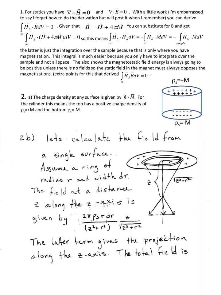
1. For statics you have and . With a little work (I’m embarrassed to say I forget how to do the derivation but will post it when I remember) you can derive : . Given that You can substitute for B and get so this means the latter is just the integration over the sample because that is only where you have magnetization. This integral is much easier because you only have to integrate over the sample and not all space. The also shows the magnetostatic field energy is always going to be positive unless there is no fields so the static field in the magnet must always opposes the magnetizations. (extra points for this that derived . rs=+M + + + + + + + + + + + + 2. a) The charge density at any surface is given by For the cylinder this means the top has a positive charge density of rs=+M and the bottom rs=-M. - - - - - - - - - - - - rs=-M
d) Inside the magnet B = HZ + 4pM where HZ is from 2b Outside the magnet B = HZ where HZ is from 2C
f) For a Hin = -4pM and Bin= Hin + 4pM = 0. This is what is expected for a uniform film with the magnetization normal to the surface.
2g Magnitude of the field inside the L=1 cm magnet Magnitude of the field inside the L=10 cm magnet Magnitude of the field outside the L=10 cm magnet Magnitude of the field outside the L=1 cm magnet Notice that for the L=10 cm magnetic the magnetic field in the magnet is very inhomogeneous and is much higher near the ends. This often results in the magnet to start to reverse at the ends where there is a large demagnetization field. 2h The 1/e distance (shown above) is about 0.8a so the radius of the magnetic gives the rough length scale over what distance the field will fall off.
3). Magnetic fields are generated by magnetic poles either surface or bulk Since the magnetization is always parallel to the surface then there are no surface charges. For the bulk charges the divergence of the defined magnetization (most easily done in cylindrical coordinates) is zero. Since there are no charges there are no fields generated. 4). For a Ni wire where L >> a the internal field within the wire when the magnetization in perpendicular wire is 2pMs. You need to overcome this field to rotate the magnetization so you need 2pMs field which for Ni (Ms= 484 emu/cm3) yielding an expected saturation field of 3040 Oe. 5). a) assume L = 6cm, a = 0.625cm then the magnetization is M = 7.45×10³/(πa2L) = 1000 emu/cc. b) The magnetic moment of a solenoid is: = 7.45 x 10³emu. For n=200 turns then i= 303.5 A c) For i=1.5 A you get m= 36.8 emu 6). Assume you can measure 10-6 emu signal is typical for a good magnetometer. If you Fe (1700 emu/cm3) on a 0.5 x 0.5 cm substrate then you can estimate the thickness of Fe to give 10-6 emu = 1700 * 0.5 * 0.5 * t. This gives a thickness t=2.35x10⁻⁹ cm or 0.024 nm. The atomic spacing for Fe is 0.144 nm so it is much less than a single monolayer of Fe. 7). a) T=300K and kB = 1.38x10⁻¹⁶ erg/K. Given a particles r=5 nm then V=4pr3/3 = 5.24x10⁻¹⁹ cm3. For particle 1, EB = K1V = 4x10⁶ ergs/cm3 V= 50.6 kBT. For particle 2 you have E= for the anisotropy. The minimum energy is for q=0 or pso Emin=0. The maximum energy is q=p/2 where Emax=(K1+K2)V . The height of the energy barrier is Emax-Emin = (K1+K2)V = 50.6 kBT the same as particle 1. A plot of the two energy barriers is shown below.
Graph of the anisotropy energy versus angle for particle 1 and 2. Notice the slight difference in energy for particle when you have higher order anisotropy. b) For particle 1 the coercive field is given by Hc = 2K1/M = 2(4x10⁶)/1000 = 8000 Oe. For particle 2 this is a tricky problem and a bit more subtle. You can solve for the energy with applied field E= and track the energy barriers. I prefer to do this graphically. Shown below this energy for applied different field. As you see in the plot to the left the energy minimum for at 180 deg has disappeared at a already by 6000 Oe, much less then the coercive field of particle 1. Shown to the right I zoom into the region where the energy barrier disappears. The barrier disappears at Hc=5850 Oe. Prior to switching you see two new minimum appear (arrows in the figure) so this indicates that the magnetization has tilted some before it reverses. Since have a particle with higher order anisotropy reverses at a lower field for the same energy barrier there is in applications to be able to control K2without much success.
c) Below is the solution from Cullity(page 221). c) Repeating this
8 a) For a uniaxial particle: HC=2K/M. K=1x10⁵ ergs/cm3 HC = 200 Oe. K=1x10⁶ergs/cm3 HC = 2000 Oe. K=1x10⁷ergs/cm3 HC = 20,000 Oe. K=1x10⁸ergs/cm3 HC = 200,000 Oe. (this is a huge number!). b) From the notes where A=1x10⁻⁶ ergs/cm K=1x10⁵ ergs/cm3R = 4.53 nm (this is not a physical number since we didn’t consider the width of the domain wall. K=1x10⁶ ergs/cm3R = 14.3 nm K=1x10⁷ ergs/cm3R = 45.3 nm K=1x10⁸ ergs/cm3R = 143.2 nm These number are too small. You need to perform a proper micromagnetic calculation that includes the width of the domain wall and the magnetic fields inside the sphere even in the domain state. c) The stability for 1 second corresponds to the particle energy KV = 20 kBT which is the rough estimate for a superparamagnetic particle. kB = 1.38x10⁻¹⁶erg/Kand T=300 K. This leads to R= (15kBT/pK)^1/3. K=1x10⁵ergs/cm3 R = 12.6 nm K=1x10⁶ergs/cm3 R = 5.8 nm K=1x10⁷ ergs/cm3 R = 2.7 nm K=1x10⁸ ergs/cm3 R = 1.3 nm d) You need to use Sharrock’s eq. where Hc0 is the value from (a) i.e. the zero temperature coercive field, tp=1 sec, the measurement time and f0 = 1 x 10¹⁰ /sec (10 GHz). You know EB/kBT at T=300 K is 20. So at 200 K it is now 30 or kBT/EB= 1/30. The quantity in the square brackets is 0.39. So at 200 K the HC values measured at 1 sec with 0.39 times the values in (a). At 100 K the kBT/EB = 1/60 so the factor in the square bracket is 0.85 so multiply the results in (a) by 0.85. e) The inverse of the time scale for switching is t-1 ~ f0exp(-EB/kBT) so t = f0-1exp(EB/kBT). F0=1x10¹⁰ and EB/kBT equals 30 at 200 K and 60 at 100 K. At 200 K, t = 1070 sec. At 100 K, t = 1.14 x 10¹⁶ sec or 363,000,000 years!
For a superparamagnetic particle with strong anisotropy there will be two states allowed, up and down. This is the same as the quantum calculation of a the Brillion function for J= ½ state. The energy of the two states are: and . The average magnetization is given by which for two states is Which differs from the simple Langevin function for a zero anisotropy particle. The curves are shown below: